Free Statistics
of Irreproducible Research!
Description of Statistical Computation | |||||||||||||||||||||
|---|---|---|---|---|---|---|---|---|---|---|---|---|---|---|---|---|---|---|---|---|---|
| Author's title | |||||||||||||||||||||
| Author | *The author of this computation has been verified* | ||||||||||||||||||||
| R Software Module | rwasp_meanplot.wasp | ||||||||||||||||||||
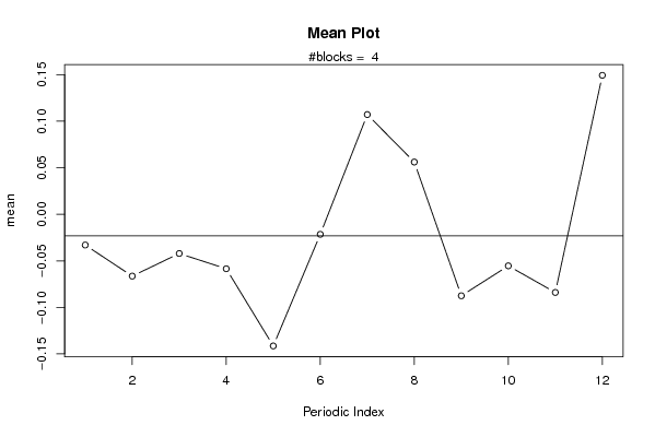
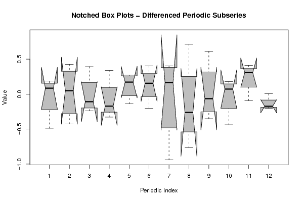
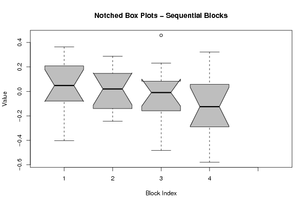
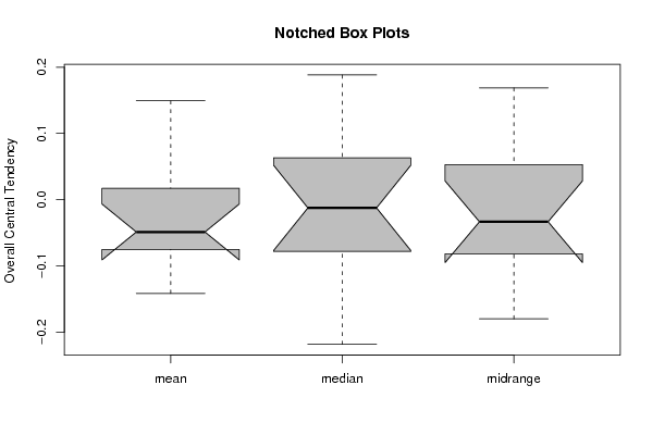
| Title produced by software | Mean Plot | ||||||||||||||||||||
| Date of computation | Tue, 01 Dec 2009 13:43:16 -0700 | ||||||||||||||||||||
| Cite this page as follows | Statistical Computations at FreeStatistics.org, Office for Research Development and Education, URL https://freestatistics.org/blog/index.php?v=date/2009/Dec/01/t1259700255yqegfhpz4smdcmj.htm/, Retrieved Wed, 09 Jul 2025 22:58:30 +0000 | ||||||||||||||||||||
| Statistical Computations at FreeStatistics.org, Office for Research Development and Education, URL https://freestatistics.org/blog/index.php?pk=62252, Retrieved Wed, 09 Jul 2025 22:58:30 +0000 | |||||||||||||||||||||
| QR Codes: | |||||||||||||||||||||
|
| |||||||||||||||||||||
| Original text written by user: | |||||||||||||||||||||
| IsPrivate? | No (this computation is public) | ||||||||||||||||||||
| User-defined keywords | |||||||||||||||||||||
| Estimated Impact | 254 | ||||||||||||||||||||
Tree of Dependent Computations | |||||||||||||||||||||
| Family? (F = Feedback message, R = changed R code, M = changed R Module, P = changed Parameters, D = changed Data) | |||||||||||||||||||||
| - [Univariate Data Series] [data set] [2008-12-01 19:54:57] [b98453cac15ba1066b407e146608df68] - RMP [ARIMA Backward Selection] [] [2009-11-27 14:53:14] [b98453cac15ba1066b407e146608df68] - D [ARIMA Backward Selection] [BBWS9-Arimabackward1] [2009-12-01 20:26:03] [408e92805dcb18620260f240a7fb9d53] - RM D [Harrell-Davis Quantiles] [BBWS9-Harolddavis] [2009-12-01 20:39:11] [408e92805dcb18620260f240a7fb9d53] - RM [Mean Plot] [BBWS9-Meanplot] [2009-12-01 20:43:16] [b32ceebc68d054278e6bda97f3d57f91] [Current] - PD [Mean Plot] [W9: Mean plot] [2009-12-02 10:46:07] [03d5b865e91ca35b5a5d21b8d6da5aba] - D [Mean Plot] [WS9 Mean Plot Yt ...] [2009-12-04 16:04:10] [1b4c3bbe3f2ba180dd536c5a6a81a8e6] - D [Mean Plot] [W9.9] [2009-12-04 17:33:15] [d31db4f83c6a129f6d3e47077769e868] - PD [Mean Plot] [workshop 9] [2009-12-04 11:57:21] [28d531aeb5ea2ff1b676cbab66947a19] - D [Mean Plot] [workshop 9] [2009-12-08 21:17:21] [28d531aeb5ea2ff1b676cbab66947a19] - R PD [Mean Plot] [shw-ws9] [2009-12-04 13:33:50] [2663058f2a5dda519058ac6b2228468f] - PD [Mean Plot] [ws 9 mean plot] [2009-12-04 19:27:12] [134dc66689e3d457a82860db6471d419] - D [Mean Plot] [Paper MP IGP] [2009-12-15 20:54:47] [134dc66689e3d457a82860db6471d419] - D [Mean Plot] [Paper MP ICP] [2009-12-15 21:02:57] [134dc66689e3d457a82860db6471d419] | |||||||||||||||||||||
| Feedback Forum | |||||||||||||||||||||
Post a new message | |||||||||||||||||||||
Dataset | |||||||||||||||||||||
| Dataseries X: | |||||||||||||||||||||
-0.0349102355942728 0.00807721497901564 -0.121638609033658 0.271140172031791 0.115362521983019 0.208637719955046 0.00736333218421053 0.364107986611877 -0.401950824320542 0.208115628227064 -0.231184614403349 0.0886065933683892 -0.115016757667903 0.0105278025279736 0.238703049625312 0.0833760938194638 -0.244263809620781 0.0300469072378363 0.160888921911825 0.136128315686798 -0.178471109158176 -0.156191416101216 -0.123271475512903 0.287855689322172 0.114229814421261 -0.373596176543768 0.0534370488169519 -0.0094243656563928 -0.196264153183377 0.0544183083541583 0.458801613285757 -0.481978233278928 0.231921304283570 -0.120496663818209 -0.00860173725973467 -0.101427264965322 -0.096296702560096 0.0893328589991427 -0.338915896651276 -0.579111335739363 -0.240498095063384 -0.379196305811148 -0.198420345132734 0.206304690993777 -0.00161455539305067 -0.152996595141273 0.0272720847132301 0.322114095042851 | |||||||||||||||||||||
Tables (Output of Computation) | |||||||||||||||||||||
| |||||||||||||||||||||
Figures (Output of Computation) | |||||||||||||||||||||
Input Parameters & R Code | |||||||||||||||||||||
| Parameters (Session): | |||||||||||||||||||||
| par1 = FALSE ; par2 = 0.5 ; par3 = 1 ; par4 = 1 ; par5 = 12 ; par6 = 3 ; par7 = 1 ; par8 = 2 ; par9 = 1 ; | |||||||||||||||||||||
| Parameters (R input): | |||||||||||||||||||||
| par1 = 12 ; | |||||||||||||||||||||
| R code (references can be found in the software module): | |||||||||||||||||||||
par1 <- as.numeric(par1) | |||||||||||||||||||||