Free Statistics
of Irreproducible Research!
Description of Statistical Computation | |||||||||||||||||||||
|---|---|---|---|---|---|---|---|---|---|---|---|---|---|---|---|---|---|---|---|---|---|
| Author's title | |||||||||||||||||||||
| Author | *The author of this computation has been verified* | ||||||||||||||||||||
| R Software Module | rwasp_meanplot.wasp | ||||||||||||||||||||
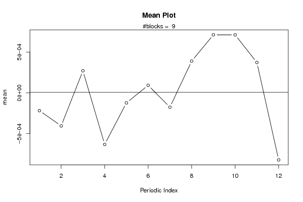
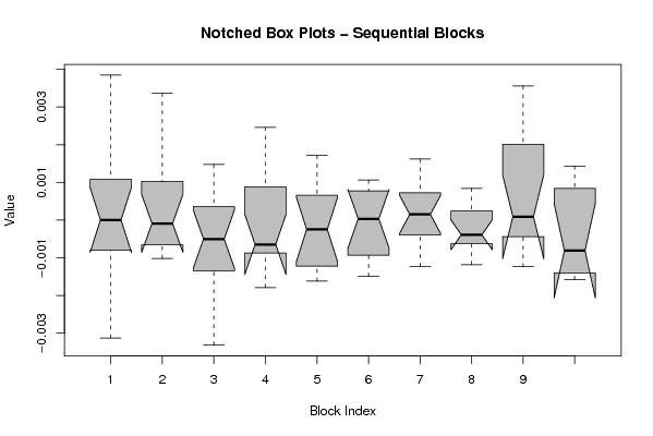
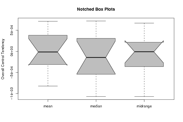
| Title produced by software | Mean Plot | ||||||||||||||||||||
| Date of computation | Fri, 04 Dec 2009 12:27:12 -0700 | ||||||||||||||||||||
| Cite this page as follows | Statistical Computations at FreeStatistics.org, Office for Research Development and Education, URL https://freestatistics.org/blog/index.php?v=date/2009/Dec/04/t1259954887fcub949eqw66104.htm/, Retrieved Mon, 15 Sep 2025 09:41:40 +0000 | ||||||||||||||||||||
| Statistical Computations at FreeStatistics.org, Office for Research Development and Education, URL https://freestatistics.org/blog/index.php?pk=64065, Retrieved Mon, 15 Sep 2025 09:41:40 +0000 | |||||||||||||||||||||
| QR Codes: | |||||||||||||||||||||
|
| |||||||||||||||||||||
| Original text written by user: | |||||||||||||||||||||
| IsPrivate? | No (this computation is public) | ||||||||||||||||||||
| User-defined keywords | |||||||||||||||||||||
| Estimated Impact | 241 | ||||||||||||||||||||
Tree of Dependent Computations | |||||||||||||||||||||
| Family? (F = Feedback message, R = changed R code, M = changed R Module, P = changed Parameters, D = changed Data) | |||||||||||||||||||||
| - [Univariate Data Series] [data set] [2008-12-01 19:54:57] [b98453cac15ba1066b407e146608df68] - RMP [ARIMA Backward Selection] [] [2009-11-27 14:53:14] [b98453cac15ba1066b407e146608df68] - D [ARIMA Backward Selection] [BBWS9-Arimabackward1] [2009-12-01 20:26:03] [408e92805dcb18620260f240a7fb9d53] - RM D [Harrell-Davis Quantiles] [BBWS9-Harolddavis] [2009-12-01 20:39:11] [408e92805dcb18620260f240a7fb9d53] - RM [Mean Plot] [BBWS9-Meanplot] [2009-12-01 20:43:16] [408e92805dcb18620260f240a7fb9d53] - R PD [Mean Plot] [shw-ws9] [2009-12-04 13:33:50] [2663058f2a5dda519058ac6b2228468f] - PD [Mean Plot] [ws 9 mean plot] [2009-12-04 19:27:12] [4f297b039e1043ebee7ff7a83b1eaaaa] [Current] - D [Mean Plot] [Paper MP IGP] [2009-12-15 20:54:47] [134dc66689e3d457a82860db6471d419] - D [Mean Plot] [Paper MP ICP] [2009-12-15 21:02:57] [134dc66689e3d457a82860db6471d419] | |||||||||||||||||||||
| Feedback Forum | |||||||||||||||||||||
Post a new message | |||||||||||||||||||||
Dataset | |||||||||||||||||||||
| Dataseries X: | |||||||||||||||||||||
-5.57188623643403e-05 0.000673127001655781 0.00253297316798237 -0.00312808800265659 6.06736685254191e-05 0.00111459533092098 -0.000554109520648384 -0.00105302564390300 0.00104708036627266 -0.000154081652574897 0.00384608131631652 -0.00119915735301702 -0.000654000489824518 0.00147251443605623 -0.000700006059835063 -0.00061908177055739 0.000837030387252926 0.00112904739358168 -0.000635971834993874 0.000438787250423991 0.00336388391216243 0.000921403408594523 -0.000666757721707773 -0.00102031957840900 -0.000796646941257639 -0.00332057539851693 -0.000182532249361493 0.000146444976543607 0.000563712163999504 -0.00101555676532265 -0.000213138748455123 -0.00116972320289465 0.000718163786614911 0.00147451936379633 -0.00186871515930147 -0.00152438264067532 -0.00079919301702642 0.00214361864863578 0.00246081566765619 -0.00105955030987362 -0.000841465941827341 -0.000224431304780554 -0.000524348696489676 0.00168130096323857 -0.00179203973258881 8.57375031507516e-05 -0.000771092454595768 -0.000903583373710958 0.000148807028873512 -0.001557405462672 0.000344209067865560 -0.00101577409715098 0.000968280070164763 -0.000691907060623672 -0.000647161091857317 0.000306078767940221 -0.00143204637452955 0.00171652552326860 0.00100568755956631 -0.00162283353151299 -5.03611946386278e-05 -0.00139199227766638 0.0008205486056255 0.00106165242946242 -0.00149168951466355 0.000113318551053342 -0.000798705188071938 0.000725657525939686 0.000996463288562474 0.000551870084508547 -0.000750413138897793 -0.00107155858159102 0.000778446826870656 -0.000420986168065270 -0.00123476222127950 5.58572848751406e-05 0.000674648736605934 -0.00070571283485043 0.000562433086011177 0.00155795278362076 0.000246475697694884 -0.000138379316298359 -0.000372926968554567 0.00161826258007914 -0.00118416871764147 -1.79064625009521e-05 -0.000530448371326978 0.000513060612174883 -0.000488611530751738 -0.000344435665802584 0.000842398928486991 -0.00078884664263527 -0.00030481479842588 -0.00072415539117241 0.000502998571283987 -0.000437715789622652 -0.000201547985612967 -0.000674925273024028 -0.000139783804754848 -0.000849121145158096 6.60224785191873e-05 0.000113764899993581 0.00159428581141906 0.00113767761833825 0.00355745661277584 0.00266114068025193 0.00242685751739785 -0.00123747069021010 0.000630850445637065 -0.000959554038128756 -0.000666732374209195 -0.00142693285098644 -0.00158022058363810 0.00143352595627639 -0.00138297408790195 0.00105401647418059 | |||||||||||||||||||||
Tables (Output of Computation) | |||||||||||||||||||||
| |||||||||||||||||||||
Figures (Output of Computation) | |||||||||||||||||||||
Input Parameters & R Code | |||||||||||||||||||||
| Parameters (Session): | |||||||||||||||||||||
| par1 = 12 ; | |||||||||||||||||||||
| Parameters (R input): | |||||||||||||||||||||
| par1 = 12 ; | |||||||||||||||||||||
| R code (references can be found in the software module): | |||||||||||||||||||||
par1 <- as.numeric(par1) | |||||||||||||||||||||