Free Statistics
of Irreproducible Research!
Description of Statistical Computation | |||||||||||||||||||||
|---|---|---|---|---|---|---|---|---|---|---|---|---|---|---|---|---|---|---|---|---|---|
| Author's title | |||||||||||||||||||||
| Author | *The author of this computation has been verified* | ||||||||||||||||||||
| R Software Module | rwasp_meanplot.wasp | ||||||||||||||||||||
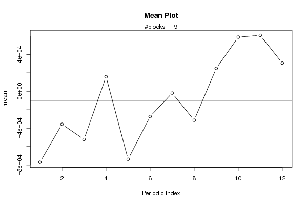
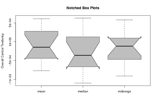
| Title produced by software | Mean Plot | ||||||||||||||||||||
| Date of computation | Tue, 15 Dec 2009 13:54:47 -0700 | ||||||||||||||||||||
| Cite this page as follows | Statistical Computations at FreeStatistics.org, Office for Research Development and Education, URL https://freestatistics.org/blog/index.php?v=date/2009/Dec/15/t1260910551mnzovxqpnv9xy16.htm/, Retrieved Mon, 15 Sep 2025 09:37:16 +0000 | ||||||||||||||||||||
| Statistical Computations at FreeStatistics.org, Office for Research Development and Education, URL https://freestatistics.org/blog/index.php?pk=68150, Retrieved Mon, 15 Sep 2025 09:37:16 +0000 | |||||||||||||||||||||
| QR Codes: | |||||||||||||||||||||
|
| |||||||||||||||||||||
| Original text written by user: | |||||||||||||||||||||
| IsPrivate? | No (this computation is public) | ||||||||||||||||||||
| User-defined keywords | |||||||||||||||||||||
| Estimated Impact | 245 | ||||||||||||||||||||
Tree of Dependent Computations | |||||||||||||||||||||
| Family? (F = Feedback message, R = changed R code, M = changed R Module, P = changed Parameters, D = changed Data) | |||||||||||||||||||||
| - [Univariate Data Series] [data set] [2008-12-01 19:54:57] [b98453cac15ba1066b407e146608df68] - RMP [ARIMA Backward Selection] [] [2009-11-27 14:53:14] [b98453cac15ba1066b407e146608df68] - D [ARIMA Backward Selection] [BBWS9-Arimabackward1] [2009-12-01 20:26:03] [408e92805dcb18620260f240a7fb9d53] - RM D [Harrell-Davis Quantiles] [BBWS9-Harolddavis] [2009-12-01 20:39:11] [408e92805dcb18620260f240a7fb9d53] - RM [Mean Plot] [BBWS9-Meanplot] [2009-12-01 20:43:16] [408e92805dcb18620260f240a7fb9d53] - R PD [Mean Plot] [shw-ws9] [2009-12-04 13:33:50] [2663058f2a5dda519058ac6b2228468f] - PD [Mean Plot] [ws 9 mean plot] [2009-12-04 19:27:12] [134dc66689e3d457a82860db6471d419] - D [Mean Plot] [Paper MP IGP] [2009-12-15 20:54:47] [4f297b039e1043ebee7ff7a83b1eaaaa] [Current] | |||||||||||||||||||||
| Feedback Forum | |||||||||||||||||||||
Post a new message | |||||||||||||||||||||
Dataset | |||||||||||||||||||||
| Dataseries X: | |||||||||||||||||||||
3.98079081276633e-05 -0.000973976133257226 9.54105981046696e-05 0.0025088460252085 -0.00317190862576495 -0.000294031330328119 0.000968982944777646 -0.000851197318024926 -0.00138793660546551 0.000768157042933171 -0.00043345520475556 0.00366870846041696 -0.00115605912816505 -0.000726387151364303 0.00158304848369840 -0.000705551333861491 -0.000686845735372371 0.000856524956680535 0.00112951149233031 -0.000633986568076334 0.000485377794173421 0.00350968792492686 0.00110875144650834 -0.000454222753280748 -0.00070519397282043 -0.000564138898205549 -0.00323625658579197 -0.000207775895461774 0.000121573704094360 0.00043576463403868 -0.00105292199456297 -0.0002403967976497 -0.00118907538442198 0.000625841684237297 0.00143341373589394 -0.00192988553325272 -0.00157492400816634 -0.000826348774317081 0.00200273506082489 0.00234881104580967 -0.00111885056021927 -0.00081068847426387 -0.000153003860193700 -0.000584636837683116 0.00160325078754813 -0.00183253836358638 -2.44819684689276e-06 -0.000771460372823094 -0.00104001978218138 4.48050729071727e-05 -0.00169203184569203 0.000174462273812442 -0.00114098465483701 0.000769566716964055 -0.000818911240646756 -0.000828750325242718 0.00018261275748915 -0.00159799022419187 0.00152164245558621 0.000884169332101304 -0.00180485032467462 -0.000145630936549182 -0.00147324017244386 0.00060792316144348 0.000905629038218515 -0.00169040652912523 -3.12105291171649e-05 -0.000906676164921031 0.000514094616829656 0.000837486441965654 0.000374199742847721 -0.000878094545087892 -0.001182893501353 0.000646111491672511 -0.000599857591795931 -0.00144802173609301 -0.000104582917017275 0.000492759150213751 -0.000931164919957729 0.000371424202406294 0.00140975891549500 6.6750425077598e-05 -0.000277340783067839 -0.000455194022166956 0.00149545439655812 -0.00131297831713598 -0.000172568590443257 -0.000606874399482126 0.000336885535519071 -0.000642830360379811 -0.000512599342982913 0.000704580414167671 -0.000945254989964433 -0.000475584476934928 -0.000848558711677428 0.000314088890732562 -0.000617706260337561 -0.000400848410183710 -0.000838652504832539 -0.000333202351853059 -0.00104162067143271 -0.000146313497017913 -8.59352300135553e-05 0.00137121135042611 0.000958241811236665 0.00339310785749926 0.00259450104170567 0.00237818486786294 -0.00116307131503507 0.000681404236029412 -0.000892729488794187 -0.000758226783340658 -0.00148062583439785 -0.00170642385731143 0.00129224214825562 -0.00154330598635992 0.000855094334823046 | |||||||||||||||||||||
Tables (Output of Computation) | |||||||||||||||||||||
| |||||||||||||||||||||
Figures (Output of Computation) | |||||||||||||||||||||
Input Parameters & R Code | |||||||||||||||||||||
| Parameters (Session): | |||||||||||||||||||||
| par1 = 12 ; | |||||||||||||||||||||
| Parameters (R input): | |||||||||||||||||||||
| par1 = 12 ; | |||||||||||||||||||||
| R code (references can be found in the software module): | |||||||||||||||||||||
par1 <- as.numeric(par1) | |||||||||||||||||||||