Free Statistics
of Irreproducible Research!
Description of Statistical Computation | |||||||||||||||||||||
|---|---|---|---|---|---|---|---|---|---|---|---|---|---|---|---|---|---|---|---|---|---|
| Author's title | |||||||||||||||||||||
| Author | *The author of this computation has been verified* | ||||||||||||||||||||
| R Software Module | rwasp_meanplot.wasp | ||||||||||||||||||||
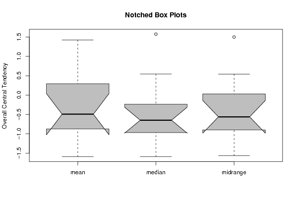
| Title produced by software | Mean Plot | ||||||||||||||||||||
| Date of computation | Fri, 04 Dec 2009 06:33:50 -0700 | ||||||||||||||||||||
| Cite this page as follows | Statistical Computations at FreeStatistics.org, Office for Research Development and Education, URL https://freestatistics.org/blog/index.php?v=date/2009/Dec/04/t1259933672tuigsbi3yna5o43.htm/, Retrieved Tue, 26 May 2026 00:12:12 +0000 | ||||||||||||||||||||
| Statistical Computations at FreeStatistics.org, Office for Research Development and Education, URL https://freestatistics.org/blog/index.php?pk=63491, Retrieved Tue, 26 May 2026 00:12:12 +0000 | |||||||||||||||||||||
| QR Codes: | |||||||||||||||||||||
|
| |||||||||||||||||||||
| Original text written by user: | |||||||||||||||||||||
| IsPrivate? | No (this computation is public) | ||||||||||||||||||||
| User-defined keywords | Workshop 9 - residu's 2 | ||||||||||||||||||||
| Estimated Impact | 438 | ||||||||||||||||||||
Tree of Dependent Computations | |||||||||||||||||||||
| Family? (F = Feedback message, R = changed R code, M = changed R Module, P = changed Parameters, D = changed Data) | |||||||||||||||||||||
| - [Univariate Data Series] [data set] [2008-12-01 19:54:57] [b98453cac15ba1066b407e146608df68] - RMP [ARIMA Backward Selection] [] [2009-11-27 14:53:14] [b98453cac15ba1066b407e146608df68] - D [ARIMA Backward Selection] [BBWS9-Arimabackward1] [2009-12-01 20:26:03] [408e92805dcb18620260f240a7fb9d53] - RM D [Harrell-Davis Quantiles] [BBWS9-Harolddavis] [2009-12-01 20:39:11] [408e92805dcb18620260f240a7fb9d53] - RM [Mean Plot] [BBWS9-Meanplot] [2009-12-01 20:43:16] [408e92805dcb18620260f240a7fb9d53] - R PD [Mean Plot] [shw-ws9] [2009-12-04 13:33:50] [5b5bced41faf164488f2c271c918b21f] [Current] - PD [Mean Plot] [ws 9 mean plot] [2009-12-04 19:27:12] [134dc66689e3d457a82860db6471d419] - D [Mean Plot] [Paper MP IGP] [2009-12-15 20:54:47] [134dc66689e3d457a82860db6471d419] - D [Mean Plot] [Paper MP ICP] [2009-12-15 21:02:57] [134dc66689e3d457a82860db6471d419] | |||||||||||||||||||||
| Feedback Forum | |||||||||||||||||||||
Post a new message | |||||||||||||||||||||
Dataset | |||||||||||||||||||||
| Dataseries X: | |||||||||||||||||||||
-0.182516799296172 -0.94944747492426 0.325776406812306 1.34843784634604 1.75851178494723 -4.42943737703812 -2.31767034001953 -2.79684843911972 1.12860275120424 0.217683629453875 -0.216346021448786 0.255354934382147 2.08016887397565 1.98907623974419 -3.52512220833211 1.92157710024745 -1.23357233233317 -0.578487095948195 5.06860933422247 -4.07661330236988 -1.08022426396436 -2.92628938204488 1.85793956152257 -0.724378886250608 -1.18764122154349 -4.95476521135668 -2.32628727835623 -0.861616376891362 0.240169843746047 -1.29423362584277 -0.405011745027942 0.234630784545567 2.02245409411938 -1.53833721759871 -1.22520941203817 -1.34782503211567 -1.09231372313534 -2.23500733525864 2.01390498049689 -0.25916025754455 -0.251975811363012 3.19306194411413 -0.520346345270884 0.263552410490847 3.6273589881661 0.757824778633043 -2.20481542891670 -0.350907792837528 | |||||||||||||||||||||
Tables (Output of Computation) | |||||||||||||||||||||
| |||||||||||||||||||||
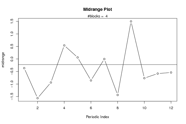
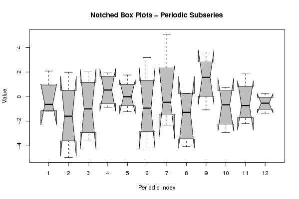
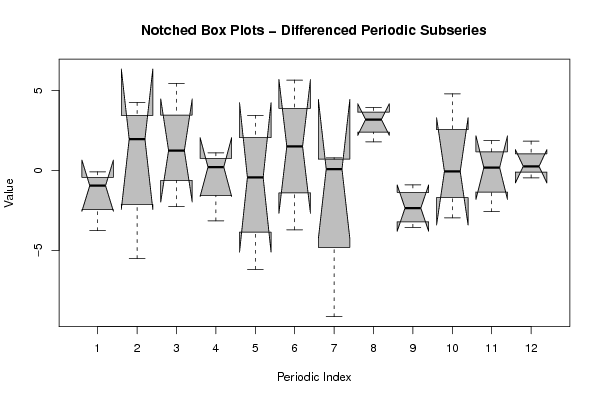
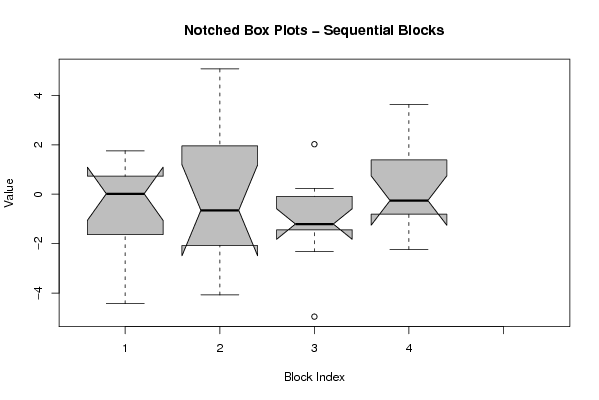
Figures (Output of Computation) | |||||||||||||||||||||
Input Parameters & R Code | |||||||||||||||||||||
| Parameters (Session): | |||||||||||||||||||||
| par1 = 0.01 ; par2 = 0.99 ; par3 = 0.005 ; | |||||||||||||||||||||
| Parameters (R input): | |||||||||||||||||||||
| par1 = 12 ; | |||||||||||||||||||||
| R code (references can be found in the software module): | |||||||||||||||||||||
par1 <- as.numeric(par1) | |||||||||||||||||||||