Repository of Reproducible Computations

Free Statistics

of Irreproducible Research!

Author's title

Author

*The author of this computation has been verified*

R Software Module

rwasp_meanplot.wasp

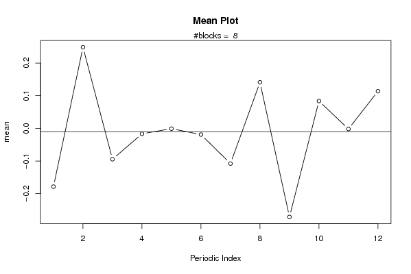
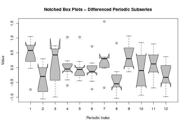
Title produced by software

Mean Plot

Date of computation

Tue, 15 Dec 2009 14:02:57 -0700

Cite this page as follows

Statistical Computations at FreeStatistics.org, Office for Research Development and Education, URL https://freestatistics.org/blog/index.php?v=date/2009/Dec/15/t1260911036d0zt0rl5o0z0dad.htm/, Retrieved Sun, 28 Apr 2024 23:14:18 +0000

Statistical Computations at FreeStatistics.org, Office for Research Development and Education, URL https://freestatistics.org/blog/index.php?pk=68162, Retrieved Sun, 28 Apr 2024 23:14:18 +0000

QR Codes:

Paste this QR Code to cite your computation.

Original text written by user:

IsPrivate?

No (this computation is public)

User-defined keywords

Estimated Impact

145

Family? (F = Feedback message, R = changed R code, M = changed R Module, P = changed Parameters, D = changed Data)

-     [Univariate Data Series] [data set] [2008-12-01 19:54:57] [b98453cac15ba1066b407e146608df68]
- RMP   [ARIMA Backward Selection] [] [2009-11-27 14:53:14] [b98453cac15ba1066b407e146608df68]
-    D    [ARIMA Backward Selection] [BBWS9-Arimabackward1] [2009-12-01 20:26:03] [408e92805dcb18620260f240a7fb9d53]
- RM D      [Harrell-Davis Quantiles] [BBWS9-Harolddavis] [2009-12-01 20:39:11] [408e92805dcb18620260f240a7fb9d53]
- RM          [Mean Plot] [BBWS9-Meanplot] [2009-12-01 20:43:16] [408e92805dcb18620260f240a7fb9d53]
- R PD          [Mean Plot] [shw-ws9] [2009-12-04 13:33:50] [2663058f2a5dda519058ac6b2228468f]
-   PD            [Mean Plot] [ws 9 mean plot] [2009-12-04 19:27:12] [134dc66689e3d457a82860db6471d419]
-    D                [Mean Plot] [Paper MP ICP] [2009-12-15 21:02:57] [4f297b039e1043ebee7ff7a83b1eaaaa] [Current]

Feedback Forum

Post a new message

Dataseries X:

Download CSV

Histogram

Boxplots

-0.350799688370536
-0.140769858461987
-0.176994002962568
0.562290817956577
0.144201690134944
-0.111030533067628
-0.243045038133344
-0.151508019282699
-0.396513842133135
0.0329753101728757
-0.0833088349918484
0.156956311022783
0.523621600794454
-0.216145977751341
-0.208014642793551
-0.341520041804527
-0.114593780635957
-0.558823753124076
0.155427432046773
0.138052779163656
-0.4090756185683
0.110316654295769
-0.250998024914370
0.329481615878391
0.346878506478169
0.323299830417798
-0.0310312875854553
-0.84926656008146
-0.77680329705359
0.250909338924582
0.0831309127438593
0.435693250316565
-0.130263895758751
-0.232129238451711
0.165342569504054
0.142248180166828
-0.280455237088636
0.155402490351535
-0.142784384867873
0.28524670566859
0.157418555269204
-0.172706911536110
-0.0149928813013760
0.306296873369522
-0.345207720981392
0.722409122191829
-0.158636568880998
-0.431031704131918
-0.308095207623409
0.447320732827413
0.447799821943335
0.0214235496574372
0.152471875346584
0.163942423990300
-0.00498382593447193
0.308356992481182
-0.230794586105762
-0.0542129596699259
-0.137751473869932
0.137775171895457
-0.208611181469940
0.530877388565287
-0.307691326359942
0.287643632777539
0.239698181689028
-0.0324235808931527
-0.110760321621385
0.187857496084540
-0.629717422499043
-0.464897710438974
0.381446921054368
0.388355710424064
-0.59380461268784
0.456215309938507
-0.35419239371042
0.278101258603134
-0.32386448817015
-0.115433965509661
-0.0483653154188056
-0.0424966476262035
-0.179962353470623
0.634520247547924
1.07894182435992
0.395987866990447
-0.219758520860607
0.361998505460662
0.660014172078838
-0.331005583090054
0.695781527796754
0.646124350414131
-0.0835481139905882
-0.763493350940545
0.0627068862169823
-0.0788278540379063
-1.01076620067800
-0.208872220642831
-0.515267639977992
0.319253920126987
-0.739240050461461
-0.0632470686715278
-0.182648154761123
-0.242076757818195
-0.704413262583499
0.851791451893186
-0.183365626294880

Summary of computational transaction
Raw Input	view raw input (R code)
Raw Output	view raw output of R engine
Computing time	2 seconds
R Server	'Gwilym Jenkins' @ 72.249.127.135

\begin{tabular}{lllllllll}
\hline
Summary of computational transaction \tabularnewline
Raw Input & view raw input (R code)  \tabularnewline
Raw Output & view raw output of R engine  \tabularnewline
Computing time & 2 seconds \tabularnewline
R Server & 'Gwilym Jenkins' @ 72.249.127.135 \tabularnewline
\hline
\end{tabular}
%Source: https://freestatistics.org/blog/index.php?pk=68162&T=0

[TABLE]
[ROW][C]Summary of computational transaction[/C][/ROW]
[ROW][C]Raw Input[/C][C]view raw input (R code) [/C][/ROW]
[ROW][C]Raw Output[/C][C]view raw output of R engine [/C][/ROW]
[ROW][C]Computing time[/C][C]2 seconds[/C][/ROW]
[ROW][C]R Server[/C][C]'Gwilym Jenkins' @ 72.249.127.135[/C][/ROW]
[/TABLE]
Source: https://freestatistics.org/blog/index.php?pk=68162&T=0

Globally Unique Identifier (entire table): ba.freestatistics.org/blog/index.php?pk=68162&T=0

As an alternative you can also use a QR Code:

The GUIDs for individual cells are displayed in the table below:

Summary of computational transaction
Raw Input	view raw input (R code)
Raw Output	view raw output of R engine
Computing time	2 seconds
R Server	'Gwilym Jenkins' @ 72.249.127.135

Figure 1

PNG link

Postscript link

PDF link

Figure 2

PNG link

Postscript link

PDF link

Figure 3

PNG link

Postscript link

PDF link

Figure 4

PNG link

Postscript link

PDF link

Figure 5

PNG link

Postscript link

PDF link

Figure 6

PNG link

Postscript link

PDF link

Figure 7

PNG link

Postscript link

PDF link

Parameters (Session):

par1 = 12 ;

Parameters (R input):

par1 = 12 ;

R code (references can be found in the software module):

par1 <- as.numeric(par1)
(n <- length(x))
(np <- floor(n / par1))
arr <- array(NA,dim=c(par1,np+1))
darr <- array(NA,dim=c(par1,np+1))
ari <- array(0,dim=par1)
dx <- diff(x)
j <- 0
for (i in 1:n)
{
j = j + 1
ari[j] = ari[j] + 1
arr[j,ari[j]] <- x[i]
darr[j,ari[j]] <- dx[i]
if (j == par1) j = 0
}
ari
arr
darr
arr.mean <- array(NA,dim=par1)
arr.median <- array(NA,dim=par1)
arr.midrange <- array(NA,dim=par1)
for (j in 1:par1)
{
arr.mean[j] <- mean(arr[j,],na.rm=TRUE)
arr.median[j] <- median(arr[j,],na.rm=TRUE)
arr.midrange[j] <- (quantile(arr[j,],0.75,na.rm=TRUE) + quantile(arr[j,],0.25,na.rm=TRUE)) / 2
}
overall.mean <- mean(x)
overall.median <- median(x)
overall.midrange <- (quantile(x,0.75) + quantile(x,0.25)) / 2
bitmap(file='plot1.png')
plot(arr.mean,type='b',ylab='mean',main='Mean Plot',xlab='Periodic Index')
mtext(paste('#blocks = ',np))
abline(overall.mean,0)
dev.off()
bitmap(file='plot2.png')
plot(arr.median,type='b',ylab='median',main='Median Plot',xlab='Periodic Index')
mtext(paste('#blocks = ',np))
abline(overall.median,0)
dev.off()
bitmap(file='plot3.png')
plot(arr.midrange,type='b',ylab='midrange',main='Midrange Plot',xlab='Periodic Index')
mtext(paste('#blocks = ',np))
abline(overall.midrange,0)
dev.off()
bitmap(file='plot4.png')
z <- data.frame(t(arr))
names(z) <- c(1:par1)
(boxplot(z,notch=TRUE,col='grey',xlab='Periodic Index',ylab='Value',main='Notched Box Plots - Periodic Subseries'))
dev.off()
bitmap(file='plot4b.png')
z <- data.frame(t(darr))
names(z) <- c(1:par1)
(boxplot(z,notch=TRUE,col='grey',xlab='Periodic Index',ylab='Value',main='Notched Box Plots - Differenced Periodic Subseries'))
dev.off()
bitmap(file='plot5.png')
z <- data.frame(arr)
names(z) <- c(1:np)
(boxplot(z,notch=TRUE,col='grey',xlab='Block Index',ylab='Value',main='Notched Box Plots - Sequential Blocks'))
dev.off()
bitmap(file='plot6.png')
z <- data.frame(cbind(arr.mean,arr.median,arr.midrange))
names(z) <- list('mean','median','midrange')
(boxplot(z,notch=TRUE,col='grey',ylab='Overall Central Tendency',main='Notched Box Plots'))
dev.off()

Free Statistics

Description of Statistical Computation

Tree of Dependent Computations

Dataset

Tables (Output of Computation)

Figures (Output of Computation)

Input Parameters & R Code