Repository of Reproducible Computations

Free Statistics

of Irreproducible Research!

Author's title

Author

*Unverified author*

R Software Module

rwasp_autocorrelation.wasp

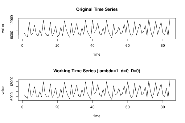
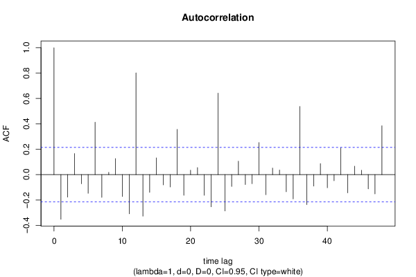
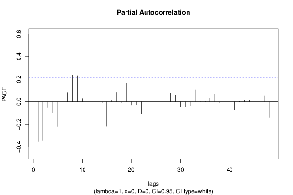
Title produced by software

(Partial) Autocorrelation Function

Date of computation

Mon, 12 Nov 2012 06:07:31 -0500

Cite this page as follows

Statistical Computations at FreeStatistics.org, Office for Research Development and Education, URL https://freestatistics.org/blog/index.php?v=date/2012/Nov/12/t1352718483o3c0nmibd3z8ub5.htm/, Retrieved Mon, 29 Apr 2024 16:33:47 +0000

Statistical Computations at FreeStatistics.org, Office for Research Development and Education, URL https://freestatistics.org/blog/index.php?pk=187765, Retrieved Mon, 29 Apr 2024 16:33:47 +0000

QR Codes:

Paste this QR Code to cite your computation.

Original text written by user:

IsPrivate?

No (this computation is public)

User-defined keywords

Estimated Impact

109

Family? (F = Feedback message, R = changed R code, M = changed R Module, P = changed Parameters, D = changed Data)

-     [Univariate Data Series] [Ontvangsten ge�nd...] [2012-10-07 17:57:08] [7e0b1fc7e94581fb4f84255f8aa2fbc5]
- RMP   [Central Tendency] [Centrummaten ontv...] [2012-10-11 15:49:27] [7e0b1fc7e94581fb4f84255f8aa2fbc5]
- R  D    [Central Tendency] [Centrummaten ontv...] [2012-10-11 15:56:24] [7e0b1fc7e94581fb4f84255f8aa2fbc5]
- RMP       [Mean Plot] [Ontvangsten schat...] [2012-10-18 14:12:08] [7e0b1fc7e94581fb4f84255f8aa2fbc5]
- RMP           [(Partial) Autocorrelation Function] [schatkist autocor...] [2012-11-12 11:07:31] [1fc6f30e88849aa85fd62e34f240f44c] [Current]
- R P             [(Partial) Autocorrelation Function] [schatkist autocor...] [2012-11-12 11:09:46] [7e0b1fc7e94581fb4f84255f8aa2fbc5] 
- RMP             [Blocked Bootstrap Plot - Central Tendency] [density plot rek ...] [2012-11-22 19:31:20] [7e0b1fc7e94581fb4f84255f8aa2fbc5] 
- R P               [Blocked Bootstrap Plot - Central Tendency] [density plot rek ...] [2012-11-22 19:33:45] [7e0b1fc7e94581fb4f84255f8aa2fbc5] 
-   P                 [Blocked Bootstrap Plot - Central Tendency] [density plot rek ...] [2012-11-22 19:35:27] [7e0b1fc7e94581fb4f84255f8aa2fbc5] 
- RMP                   [Classical Decomposition] [Classical Deompos...] [2012-12-06 18:42:10] [74be16979710d4c4e7c6647856088456] 
- R P                     [Classical Decomposition] [Classical Deompos...] [2012-12-06 18:44:34] [74be16979710d4c4e7c6647856088456] 
- RMP                       [Exponential Smoothing] [Exponential Smoot...] [2013-01-11 16:16:59] [7e0b1fc7e94581fb4f84255f8aa2fbc5] 
- RMP                 [Variability] [spreidingsmaten s...] [2012-11-30 11:19:52] [7e0b1fc7e94581fb4f84255f8aa2fbc5] 
- RMP                 [Standard Deviation Plot] [spreidingsgrafiek...] [2012-11-30 11:20:44] [7e0b1fc7e94581fb4f84255f8aa2fbc5] 
- RMP                 [Standard Deviation-Mean Plot] [spreidings- en ge...] [2012-11-30 11:21:47] [7e0b1fc7e94581fb4f84255f8aa2fbc5] 

Feedback Forum

Post a new message

Dataseries X:

Download CSV

Histogram

Boxplots

Summary of computational transaction
Raw Input	view raw input (R code)
Raw Output	view raw output of R engine
Computing time	2 seconds
R Server	'Gwilym Jenkins' @ jenkins.wessa.net

\begin{tabular}{lllllllll}
\hline
Summary of computational transaction \tabularnewline
Raw Input & view raw input (R code)  \tabularnewline
Raw Output & view raw output of R engine  \tabularnewline
Computing time & 2 seconds \tabularnewline
R Server & 'Gwilym Jenkins' @ jenkins.wessa.net \tabularnewline
\hline
\end{tabular}
%Source: https://freestatistics.org/blog/index.php?pk=187765&T=0

[TABLE]
[ROW][C]Summary of computational transaction[/C][/ROW]
[ROW][C]Raw Input[/C][C]view raw input (R code) [/C][/ROW]
[ROW][C]Raw Output[/C][C]view raw output of R engine [/C][/ROW]
[ROW][C]Computing time[/C][C]2 seconds[/C][/ROW]
[ROW][C]R Server[/C][C]'Gwilym Jenkins' @ jenkins.wessa.net[/C][/ROW]
[/TABLE]
Source: https://freestatistics.org/blog/index.php?pk=187765&T=0

Globally Unique Identifier (entire table): ba.freestatistics.org/blog/index.php?pk=187765&T=0

As an alternative you can also use a QR Code:

The GUIDs for individual cells are displayed in the table below:

Summary of computational transaction
Raw Input	view raw input (R code)
Raw Output	view raw output of R engine
Computing time	2 seconds
R Server	'Gwilym Jenkins' @ jenkins.wessa.net

Autocorrelation Function
Time lag k	ACF(k)	T-STAT	P-value
1	-0.352132	-3.2273	0.000891
2	-0.177368	-1.6256	0.05389
3	0.166303	1.5242	0.065608
4	-0.072234	-0.662	0.25488
5	-0.147435	-1.3513	0.090119
6	0.413396	3.7888	0.000142
7	-0.179389	-1.6441	0.051944
8	0.018073	0.1656	0.43442
9	0.126317	1.1577	0.125131
10	-0.172328	-1.5794	0.059
11	-0.309425	-2.8359	0.002862
12	0.802289	7.3531	0
13	-0.327515	-3.0017	0.001767
14	-0.14025	-1.2854	0.10109
15	0.13221	1.2117	0.114508
16	-0.081364	-0.7457	0.22896
17	-0.097588	-0.8944	0.18683
18	0.356284	3.2654	0.000792
19	-0.163209	-1.4958	0.069223
20	0.03465	0.3176	0.375797
21	0.055755	0.511	0.305345
22	-0.162645	-1.4907	0.069897
23	-0.253652	-2.3248	0.011249
24	0.642415	5.8878	0
25	-0.286423	-2.6251	0.005145
26	-0.093843	-0.8601	0.196096
27	0.105495	0.9669	0.168191
28	-0.078837	-0.7226	0.23598
29	-0.07172	-0.6573	0.256385
30	0.2526	2.3151	0.011523
31	-0.158332	-1.4511	0.075233
32	0.0518	0.4748	0.318096
33	0.036137	0.3312	0.370658
34	-0.135216	-1.2393	0.109347
35	-0.191957	-1.7593	0.041082
36	0.537344	4.9248	2e-06
37	-0.236347	-2.1662	0.016567
38	-0.090857	-0.8327	0.203684
39	0.087202	0.7992	0.213208
40	-0.103796	-0.9513	0.172089
41	-0.048154	-0.4413	0.330051
42	0.211382	1.9374	0.028032
43	-0.144048	-1.3202	0.095174
44	0.066758	0.6118	0.271146
45	0.034276	0.3141	0.377095
46	-0.112473	-1.0308	0.15279
47	-0.152098	-1.394	0.083496
48	0.38485	3.5272	0.000342

\begin{tabular}{lllllllll}
\hline
Autocorrelation Function \tabularnewline
Time lag k & ACF(k) & T-STAT & P-value \tabularnewline
1 & -0.352132 & -3.2273 & 0.000891 \tabularnewline
2 & -0.177368 & -1.6256 & 0.05389 \tabularnewline
3 & 0.166303 & 1.5242 & 0.065608 \tabularnewline
4 & -0.072234 & -0.662 & 0.25488 \tabularnewline
5 & -0.147435 & -1.3513 & 0.090119 \tabularnewline
6 & 0.413396 & 3.7888 & 0.000142 \tabularnewline
7 & -0.179389 & -1.6441 & 0.051944 \tabularnewline
8 & 0.018073 & 0.1656 & 0.43442 \tabularnewline
9 & 0.126317 & 1.1577 & 0.125131 \tabularnewline
10 & -0.172328 & -1.5794 & 0.059 \tabularnewline
11 & -0.309425 & -2.8359 & 0.002862 \tabularnewline
12 & 0.802289 & 7.3531 & 0 \tabularnewline
13 & -0.327515 & -3.0017 & 0.001767 \tabularnewline
14 & -0.14025 & -1.2854 & 0.10109 \tabularnewline
15 & 0.13221 & 1.2117 & 0.114508 \tabularnewline
16 & -0.081364 & -0.7457 & 0.22896 \tabularnewline
17 & -0.097588 & -0.8944 & 0.18683 \tabularnewline
18 & 0.356284 & 3.2654 & 0.000792 \tabularnewline
19 & -0.163209 & -1.4958 & 0.069223 \tabularnewline
20 & 0.03465 & 0.3176 & 0.375797 \tabularnewline
21 & 0.055755 & 0.511 & 0.305345 \tabularnewline
22 & -0.162645 & -1.4907 & 0.069897 \tabularnewline
23 & -0.253652 & -2.3248 & 0.011249 \tabularnewline
24 & 0.642415 & 5.8878 & 0 \tabularnewline
25 & -0.286423 & -2.6251 & 0.005145 \tabularnewline
26 & -0.093843 & -0.8601 & 0.196096 \tabularnewline
27 & 0.105495 & 0.9669 & 0.168191 \tabularnewline
28 & -0.078837 & -0.7226 & 0.23598 \tabularnewline
29 & -0.07172 & -0.6573 & 0.256385 \tabularnewline
30 & 0.2526 & 2.3151 & 0.011523 \tabularnewline
31 & -0.158332 & -1.4511 & 0.075233 \tabularnewline
32 & 0.0518 & 0.4748 & 0.318096 \tabularnewline
33 & 0.036137 & 0.3312 & 0.370658 \tabularnewline
34 & -0.135216 & -1.2393 & 0.109347 \tabularnewline
35 & -0.191957 & -1.7593 & 0.041082 \tabularnewline
36 & 0.537344 & 4.9248 & 2e-06 \tabularnewline
37 & -0.236347 & -2.1662 & 0.016567 \tabularnewline
38 & -0.090857 & -0.8327 & 0.203684 \tabularnewline
39 & 0.087202 & 0.7992 & 0.213208 \tabularnewline
40 & -0.103796 & -0.9513 & 0.172089 \tabularnewline
41 & -0.048154 & -0.4413 & 0.330051 \tabularnewline
42 & 0.211382 & 1.9374 & 0.028032 \tabularnewline
43 & -0.144048 & -1.3202 & 0.095174 \tabularnewline
44 & 0.066758 & 0.6118 & 0.271146 \tabularnewline
45 & 0.034276 & 0.3141 & 0.377095 \tabularnewline
46 & -0.112473 & -1.0308 & 0.15279 \tabularnewline
47 & -0.152098 & -1.394 & 0.083496 \tabularnewline
48 & 0.38485 & 3.5272 & 0.000342 \tabularnewline
\hline
\end{tabular}
%Source: https://freestatistics.org/blog/index.php?pk=187765&T=1

[TABLE]
[ROW][C]Autocorrelation Function[/C][/ROW]
[ROW][C]Time lag k[/C][C]ACF(k)[/C][C]T-STAT[/C][C]P-value[/C][/ROW]
[ROW][C]1[/C][C]-0.352132[/C][C]-3.2273[/C][C]0.000891[/C][/ROW]
[ROW][C]2[/C][C]-0.177368[/C][C]-1.6256[/C][C]0.05389[/C][/ROW]
[ROW][C]3[/C][C]0.166303[/C][C]1.5242[/C][C]0.065608[/C][/ROW]
[ROW][C]4[/C][C]-0.072234[/C][C]-0.662[/C][C]0.25488[/C][/ROW]
[ROW][C]5[/C][C]-0.147435[/C][C]-1.3513[/C][C]0.090119[/C][/ROW]
[ROW][C]6[/C][C]0.413396[/C][C]3.7888[/C][C]0.000142[/C][/ROW]
[ROW][C]7[/C][C]-0.179389[/C][C]-1.6441[/C][C]0.051944[/C][/ROW]
[ROW][C]8[/C][C]0.018073[/C][C]0.1656[/C][C]0.43442[/C][/ROW]
[ROW][C]9[/C][C]0.126317[/C][C]1.1577[/C][C]0.125131[/C][/ROW]
[ROW][C]10[/C][C]-0.172328[/C][C]-1.5794[/C][C]0.059[/C][/ROW]
[ROW][C]11[/C][C]-0.309425[/C][C]-2.8359[/C][C]0.002862[/C][/ROW]
[ROW][C]12[/C][C]0.802289[/C][C]7.3531[/C][C]0[/C][/ROW]
[ROW][C]13[/C][C]-0.327515[/C][C]-3.0017[/C][C]0.001767[/C][/ROW]
[ROW][C]14[/C][C]-0.14025[/C][C]-1.2854[/C][C]0.10109[/C][/ROW]
[ROW][C]15[/C][C]0.13221[/C][C]1.2117[/C][C]0.114508[/C][/ROW]
[ROW][C]16[/C][C]-0.081364[/C][C]-0.7457[/C][C]0.22896[/C][/ROW]
[ROW][C]17[/C][C]-0.097588[/C][C]-0.8944[/C][C]0.18683[/C][/ROW]
[ROW][C]18[/C][C]0.356284[/C][C]3.2654[/C][C]0.000792[/C][/ROW]
[ROW][C]19[/C][C]-0.163209[/C][C]-1.4958[/C][C]0.069223[/C][/ROW]
[ROW][C]20[/C][C]0.03465[/C][C]0.3176[/C][C]0.375797[/C][/ROW]
[ROW][C]21[/C][C]0.055755[/C][C]0.511[/C][C]0.305345[/C][/ROW]
[ROW][C]22[/C][C]-0.162645[/C][C]-1.4907[/C][C]0.069897[/C][/ROW]
[ROW][C]23[/C][C]-0.253652[/C][C]-2.3248[/C][C]0.011249[/C][/ROW]
[ROW][C]24[/C][C]0.642415[/C][C]5.8878[/C][C]0[/C][/ROW]
[ROW][C]25[/C][C]-0.286423[/C][C]-2.6251[/C][C]0.005145[/C][/ROW]
[ROW][C]26[/C][C]-0.093843[/C][C]-0.8601[/C][C]0.196096[/C][/ROW]
[ROW][C]27[/C][C]0.105495[/C][C]0.9669[/C][C]0.168191[/C][/ROW]
[ROW][C]28[/C][C]-0.078837[/C][C]-0.7226[/C][C]0.23598[/C][/ROW]
[ROW][C]29[/C][C]-0.07172[/C][C]-0.6573[/C][C]0.256385[/C][/ROW]
[ROW][C]30[/C][C]0.2526[/C][C]2.3151[/C][C]0.011523[/C][/ROW]
[ROW][C]31[/C][C]-0.158332[/C][C]-1.4511[/C][C]0.075233[/C][/ROW]
[ROW][C]32[/C][C]0.0518[/C][C]0.4748[/C][C]0.318096[/C][/ROW]
[ROW][C]33[/C][C]0.036137[/C][C]0.3312[/C][C]0.370658[/C][/ROW]
[ROW][C]34[/C][C]-0.135216[/C][C]-1.2393[/C][C]0.109347[/C][/ROW]
[ROW][C]35[/C][C]-0.191957[/C][C]-1.7593[/C][C]0.041082[/C][/ROW]
[ROW][C]36[/C][C]0.537344[/C][C]4.9248[/C][C]2e-06[/C][/ROW]
[ROW][C]37[/C][C]-0.236347[/C][C]-2.1662[/C][C]0.016567[/C][/ROW]
[ROW][C]38[/C][C]-0.090857[/C][C]-0.8327[/C][C]0.203684[/C][/ROW]
[ROW][C]39[/C][C]0.087202[/C][C]0.7992[/C][C]0.213208[/C][/ROW]
[ROW][C]40[/C][C]-0.103796[/C][C]-0.9513[/C][C]0.172089[/C][/ROW]
[ROW][C]41[/C][C]-0.048154[/C][C]-0.4413[/C][C]0.330051[/C][/ROW]
[ROW][C]42[/C][C]0.211382[/C][C]1.9374[/C][C]0.028032[/C][/ROW]
[ROW][C]43[/C][C]-0.144048[/C][C]-1.3202[/C][C]0.095174[/C][/ROW]
[ROW][C]44[/C][C]0.066758[/C][C]0.6118[/C][C]0.271146[/C][/ROW]
[ROW][C]45[/C][C]0.034276[/C][C]0.3141[/C][C]0.377095[/C][/ROW]
[ROW][C]46[/C][C]-0.112473[/C][C]-1.0308[/C][C]0.15279[/C][/ROW]
[ROW][C]47[/C][C]-0.152098[/C][C]-1.394[/C][C]0.083496[/C][/ROW]
[ROW][C]48[/C][C]0.38485[/C][C]3.5272[/C][C]0.000342[/C][/ROW]
[/TABLE]
Source: https://freestatistics.org/blog/index.php?pk=187765&T=1

Globally Unique Identifier (entire table): ba.freestatistics.org/blog/index.php?pk=187765&T=1

As an alternative you can also use a QR Code:

The GUIDs for individual cells are displayed in the table below:

Autocorrelation Function
Time lag k	ACF(k)	T-STAT	P-value
1	-0.352132	-3.2273	0.000891
2	-0.177368	-1.6256	0.05389
3	0.166303	1.5242	0.065608
4	-0.072234	-0.662	0.25488
5	-0.147435	-1.3513	0.090119
6	0.413396	3.7888	0.000142
7	-0.179389	-1.6441	0.051944
8	0.018073	0.1656	0.43442
9	0.126317	1.1577	0.125131
10	-0.172328	-1.5794	0.059
11	-0.309425	-2.8359	0.002862
12	0.802289	7.3531	0
13	-0.327515	-3.0017	0.001767
14	-0.14025	-1.2854	0.10109
15	0.13221	1.2117	0.114508
16	-0.081364	-0.7457	0.22896
17	-0.097588	-0.8944	0.18683
18	0.356284	3.2654	0.000792
19	-0.163209	-1.4958	0.069223
20	0.03465	0.3176	0.375797
21	0.055755	0.511	0.305345
22	-0.162645	-1.4907	0.069897
23	-0.253652	-2.3248	0.011249
24	0.642415	5.8878	0
25	-0.286423	-2.6251	0.005145
26	-0.093843	-0.8601	0.196096
27	0.105495	0.9669	0.168191
28	-0.078837	-0.7226	0.23598
29	-0.07172	-0.6573	0.256385
30	0.2526	2.3151	0.011523
31	-0.158332	-1.4511	0.075233
32	0.0518	0.4748	0.318096
33	0.036137	0.3312	0.370658
34	-0.135216	-1.2393	0.109347
35	-0.191957	-1.7593	0.041082
36	0.537344	4.9248	2e-06
37	-0.236347	-2.1662	0.016567
38	-0.090857	-0.8327	0.203684
39	0.087202	0.7992	0.213208
40	-0.103796	-0.9513	0.172089
41	-0.048154	-0.4413	0.330051
42	0.211382	1.9374	0.028032
43	-0.144048	-1.3202	0.095174
44	0.066758	0.6118	0.271146
45	0.034276	0.3141	0.377095
46	-0.112473	-1.0308	0.15279
47	-0.152098	-1.394	0.083496
48	0.38485	3.5272	0.000342

Partial Autocorrelation Function
Time lag k	PACF(k)	T-STAT	P-value
1	-0.352132	-3.2273	0.000891
2	-0.344023	-3.153	0.001121
3	-0.050214	-0.4602	0.323274
4	-0.095499	-0.8753	0.191965
5	-0.218842	-2.0057	0.024052
6	0.308511	2.8275	0.002931
7	0.081837	0.75	0.227661
8	0.234055	2.1452	0.017414
9	0.230856	2.1158	0.01866
10	0.026048	0.2387	0.405945
11	-0.465104	-4.2628	2.6e-05
12	0.60214	5.5187	0
13	0.013859	0.127	0.449615
14	-0.008197	-0.0751	0.470145
15	-0.217029	-1.9891	0.024972
16	0.010447	0.0957	0.461976
17	0.082955	0.7603	0.224604
18	-0.010701	-0.0981	0.461053
19	0.16307	1.4946	0.069388
20	-0.030331	-0.278	0.390851
21	-0.02997	-0.2747	0.39212
22	-0.105037	-0.9627	0.169235
23	-0.013591	-0.1246	0.450582
24	-0.074691	-0.6846	0.247754
25	-0.121297	-1.1117	0.134719
26	-0.046186	-0.4233	0.336578
27	-0.029474	-0.2701	0.393859
28	0.077569	0.7109	0.239547
29	0.061756	0.566	0.286452
30	-0.046417	-0.4254	0.33581
31	-0.044878	-0.4113	0.340946
32	-0.036833	-0.3376	0.368262
33	0.10587	0.9703	0.167337
34	0.002818	0.0258	0.489728
35	0.002432	0.0223	0.491137
36	0.030583	0.2803	0.38997
37	0.066569	0.6101	0.271717
38	-0.008757	-0.0803	0.468112
39	0.016272	0.1491	0.440902
40	-0.088556	-0.8116	0.209648
41	-0.073061	-0.6696	0.252469
42	0.002673	0.0245	0.490258
43	0.011841	0.1085	0.456921
44	0.013813	0.1266	0.449781
45	-0.021174	-0.1941	0.423298
46	0.072608	0.6655	0.253788
47	0.054903	0.5032	0.308072
48	-0.141012	-1.2924	0.099882

\begin{tabular}{lllllllll}
\hline
Partial Autocorrelation Function \tabularnewline
Time lag k & PACF(k) & T-STAT & P-value \tabularnewline
1 & -0.352132 & -3.2273 & 0.000891 \tabularnewline
2 & -0.344023 & -3.153 & 0.001121 \tabularnewline
3 & -0.050214 & -0.4602 & 0.323274 \tabularnewline
4 & -0.095499 & -0.8753 & 0.191965 \tabularnewline
5 & -0.218842 & -2.0057 & 0.024052 \tabularnewline
6 & 0.308511 & 2.8275 & 0.002931 \tabularnewline
7 & 0.081837 & 0.75 & 0.227661 \tabularnewline
8 & 0.234055 & 2.1452 & 0.017414 \tabularnewline
9 & 0.230856 & 2.1158 & 0.01866 \tabularnewline
10 & 0.026048 & 0.2387 & 0.405945 \tabularnewline
11 & -0.465104 & -4.2628 & 2.6e-05 \tabularnewline
12 & 0.60214 & 5.5187 & 0 \tabularnewline
13 & 0.013859 & 0.127 & 0.449615 \tabularnewline
14 & -0.008197 & -0.0751 & 0.470145 \tabularnewline
15 & -0.217029 & -1.9891 & 0.024972 \tabularnewline
16 & 0.010447 & 0.0957 & 0.461976 \tabularnewline
17 & 0.082955 & 0.7603 & 0.224604 \tabularnewline
18 & -0.010701 & -0.0981 & 0.461053 \tabularnewline
19 & 0.16307 & 1.4946 & 0.069388 \tabularnewline
20 & -0.030331 & -0.278 & 0.390851 \tabularnewline
21 & -0.02997 & -0.2747 & 0.39212 \tabularnewline
22 & -0.105037 & -0.9627 & 0.169235 \tabularnewline
23 & -0.013591 & -0.1246 & 0.450582 \tabularnewline
24 & -0.074691 & -0.6846 & 0.247754 \tabularnewline
25 & -0.121297 & -1.1117 & 0.134719 \tabularnewline
26 & -0.046186 & -0.4233 & 0.336578 \tabularnewline
27 & -0.029474 & -0.2701 & 0.393859 \tabularnewline
28 & 0.077569 & 0.7109 & 0.239547 \tabularnewline
29 & 0.061756 & 0.566 & 0.286452 \tabularnewline
30 & -0.046417 & -0.4254 & 0.33581 \tabularnewline
31 & -0.044878 & -0.4113 & 0.340946 \tabularnewline
32 & -0.036833 & -0.3376 & 0.368262 \tabularnewline
33 & 0.10587 & 0.9703 & 0.167337 \tabularnewline
34 & 0.002818 & 0.0258 & 0.489728 \tabularnewline
35 & 0.002432 & 0.0223 & 0.491137 \tabularnewline
36 & 0.030583 & 0.2803 & 0.38997 \tabularnewline
37 & 0.066569 & 0.6101 & 0.271717 \tabularnewline
38 & -0.008757 & -0.0803 & 0.468112 \tabularnewline
39 & 0.016272 & 0.1491 & 0.440902 \tabularnewline
40 & -0.088556 & -0.8116 & 0.209648 \tabularnewline
41 & -0.073061 & -0.6696 & 0.252469 \tabularnewline
42 & 0.002673 & 0.0245 & 0.490258 \tabularnewline
43 & 0.011841 & 0.1085 & 0.456921 \tabularnewline
44 & 0.013813 & 0.1266 & 0.449781 \tabularnewline
45 & -0.021174 & -0.1941 & 0.423298 \tabularnewline
46 & 0.072608 & 0.6655 & 0.253788 \tabularnewline
47 & 0.054903 & 0.5032 & 0.308072 \tabularnewline
48 & -0.141012 & -1.2924 & 0.099882 \tabularnewline
\hline
\end{tabular}
%Source: https://freestatistics.org/blog/index.php?pk=187765&T=2

[TABLE]
[ROW][C]Partial Autocorrelation Function[/C][/ROW]
[ROW][C]Time lag k[/C][C]PACF(k)[/C][C]T-STAT[/C][C]P-value[/C][/ROW]
[ROW][C]1[/C][C]-0.352132[/C][C]-3.2273[/C][C]0.000891[/C][/ROW]
[ROW][C]2[/C][C]-0.344023[/C][C]-3.153[/C][C]0.001121[/C][/ROW]
[ROW][C]3[/C][C]-0.050214[/C][C]-0.4602[/C][C]0.323274[/C][/ROW]
[ROW][C]4[/C][C]-0.095499[/C][C]-0.8753[/C][C]0.191965[/C][/ROW]
[ROW][C]5[/C][C]-0.218842[/C][C]-2.0057[/C][C]0.024052[/C][/ROW]
[ROW][C]6[/C][C]0.308511[/C][C]2.8275[/C][C]0.002931[/C][/ROW]
[ROW][C]7[/C][C]0.081837[/C][C]0.75[/C][C]0.227661[/C][/ROW]
[ROW][C]8[/C][C]0.234055[/C][C]2.1452[/C][C]0.017414[/C][/ROW]
[ROW][C]9[/C][C]0.230856[/C][C]2.1158[/C][C]0.01866[/C][/ROW]
[ROW][C]10[/C][C]0.026048[/C][C]0.2387[/C][C]0.405945[/C][/ROW]
[ROW][C]11[/C][C]-0.465104[/C][C]-4.2628[/C][C]2.6e-05[/C][/ROW]
[ROW][C]12[/C][C]0.60214[/C][C]5.5187[/C][C]0[/C][/ROW]
[ROW][C]13[/C][C]0.013859[/C][C]0.127[/C][C]0.449615[/C][/ROW]
[ROW][C]14[/C][C]-0.008197[/C][C]-0.0751[/C][C]0.470145[/C][/ROW]
[ROW][C]15[/C][C]-0.217029[/C][C]-1.9891[/C][C]0.024972[/C][/ROW]
[ROW][C]16[/C][C]0.010447[/C][C]0.0957[/C][C]0.461976[/C][/ROW]
[ROW][C]17[/C][C]0.082955[/C][C]0.7603[/C][C]0.224604[/C][/ROW]
[ROW][C]18[/C][C]-0.010701[/C][C]-0.0981[/C][C]0.461053[/C][/ROW]
[ROW][C]19[/C][C]0.16307[/C][C]1.4946[/C][C]0.069388[/C][/ROW]
[ROW][C]20[/C][C]-0.030331[/C][C]-0.278[/C][C]0.390851[/C][/ROW]
[ROW][C]21[/C][C]-0.02997[/C][C]-0.2747[/C][C]0.39212[/C][/ROW]
[ROW][C]22[/C][C]-0.105037[/C][C]-0.9627[/C][C]0.169235[/C][/ROW]
[ROW][C]23[/C][C]-0.013591[/C][C]-0.1246[/C][C]0.450582[/C][/ROW]
[ROW][C]24[/C][C]-0.074691[/C][C]-0.6846[/C][C]0.247754[/C][/ROW]
[ROW][C]25[/C][C]-0.121297[/C][C]-1.1117[/C][C]0.134719[/C][/ROW]
[ROW][C]26[/C][C]-0.046186[/C][C]-0.4233[/C][C]0.336578[/C][/ROW]
[ROW][C]27[/C][C]-0.029474[/C][C]-0.2701[/C][C]0.393859[/C][/ROW]
[ROW][C]28[/C][C]0.077569[/C][C]0.7109[/C][C]0.239547[/C][/ROW]
[ROW][C]29[/C][C]0.061756[/C][C]0.566[/C][C]0.286452[/C][/ROW]
[ROW][C]30[/C][C]-0.046417[/C][C]-0.4254[/C][C]0.33581[/C][/ROW]
[ROW][C]31[/C][C]-0.044878[/C][C]-0.4113[/C][C]0.340946[/C][/ROW]
[ROW][C]32[/C][C]-0.036833[/C][C]-0.3376[/C][C]0.368262[/C][/ROW]
[ROW][C]33[/C][C]0.10587[/C][C]0.9703[/C][C]0.167337[/C][/ROW]
[ROW][C]34[/C][C]0.002818[/C][C]0.0258[/C][C]0.489728[/C][/ROW]
[ROW][C]35[/C][C]0.002432[/C][C]0.0223[/C][C]0.491137[/C][/ROW]
[ROW][C]36[/C][C]0.030583[/C][C]0.2803[/C][C]0.38997[/C][/ROW]
[ROW][C]37[/C][C]0.066569[/C][C]0.6101[/C][C]0.271717[/C][/ROW]
[ROW][C]38[/C][C]-0.008757[/C][C]-0.0803[/C][C]0.468112[/C][/ROW]
[ROW][C]39[/C][C]0.016272[/C][C]0.1491[/C][C]0.440902[/C][/ROW]
[ROW][C]40[/C][C]-0.088556[/C][C]-0.8116[/C][C]0.209648[/C][/ROW]
[ROW][C]41[/C][C]-0.073061[/C][C]-0.6696[/C][C]0.252469[/C][/ROW]
[ROW][C]42[/C][C]0.002673[/C][C]0.0245[/C][C]0.490258[/C][/ROW]
[ROW][C]43[/C][C]0.011841[/C][C]0.1085[/C][C]0.456921[/C][/ROW]
[ROW][C]44[/C][C]0.013813[/C][C]0.1266[/C][C]0.449781[/C][/ROW]
[ROW][C]45[/C][C]-0.021174[/C][C]-0.1941[/C][C]0.423298[/C][/ROW]
[ROW][C]46[/C][C]0.072608[/C][C]0.6655[/C][C]0.253788[/C][/ROW]
[ROW][C]47[/C][C]0.054903[/C][C]0.5032[/C][C]0.308072[/C][/ROW]
[ROW][C]48[/C][C]-0.141012[/C][C]-1.2924[/C][C]0.099882[/C][/ROW]
[/TABLE]
Source: https://freestatistics.org/blog/index.php?pk=187765&T=2

Globally Unique Identifier (entire table): ba.freestatistics.org/blog/index.php?pk=187765&T=2

As an alternative you can also use a QR Code:

The GUIDs for individual cells are displayed in the table below:

Partial Autocorrelation Function
Time lag k	PACF(k)	T-STAT	P-value
1	-0.352132	-3.2273	0.000891
2	-0.344023	-3.153	0.001121
3	-0.050214	-0.4602	0.323274
4	-0.095499	-0.8753	0.191965
5	-0.218842	-2.0057	0.024052
6	0.308511	2.8275	0.002931
7	0.081837	0.75	0.227661
8	0.234055	2.1452	0.017414
9	0.230856	2.1158	0.01866
10	0.026048	0.2387	0.405945
11	-0.465104	-4.2628	2.6e-05
12	0.60214	5.5187	0
13	0.013859	0.127	0.449615
14	-0.008197	-0.0751	0.470145
15	-0.217029	-1.9891	0.024972
16	0.010447	0.0957	0.461976
17	0.082955	0.7603	0.224604
18	-0.010701	-0.0981	0.461053
19	0.16307	1.4946	0.069388
20	-0.030331	-0.278	0.390851
21	-0.02997	-0.2747	0.39212
22	-0.105037	-0.9627	0.169235
23	-0.013591	-0.1246	0.450582
24	-0.074691	-0.6846	0.247754
25	-0.121297	-1.1117	0.134719
26	-0.046186	-0.4233	0.336578
27	-0.029474	-0.2701	0.393859
28	0.077569	0.7109	0.239547
29	0.061756	0.566	0.286452
30	-0.046417	-0.4254	0.33581
31	-0.044878	-0.4113	0.340946
32	-0.036833	-0.3376	0.368262
33	0.10587	0.9703	0.167337
34	0.002818	0.0258	0.489728
35	0.002432	0.0223	0.491137
36	0.030583	0.2803	0.38997
37	0.066569	0.6101	0.271717
38	-0.008757	-0.0803	0.468112
39	0.016272	0.1491	0.440902
40	-0.088556	-0.8116	0.209648
41	-0.073061	-0.6696	0.252469
42	0.002673	0.0245	0.490258
43	0.011841	0.1085	0.456921
44	0.013813	0.1266	0.449781
45	-0.021174	-0.1941	0.423298
46	0.072608	0.6655	0.253788
47	0.054903	0.5032	0.308072
48	-0.141012	-1.2924	0.099882

Figure 1

PNG link

Postscript link

PDF link

Figure 2

PNG link

Postscript link

PDF link

Figure 3

PNG link

Postscript link

PDF link

Parameters (Session):

par1 = 48 ; par2 = 1 ; par3 = 0 ; par4 = 0 ; par5 = 12 ; par6 = White Noise ; par7 = 0.95 ;

Parameters (R input):

par1 = 48 ; par2 = 1 ; par3 = 0 ; par4 = 0 ; par5 = 12 ; par6 = White Noise ; par7 = 0.95 ; par8 = ;

R code (references can be found in the software module):

par8 <- ''
par7 <- '0.95'
par6 <- 'White Noise'
par5 <- '12'
par4 <- '0'
par3 <- '0'
par2 <- '1'
par1 <- 'Default'
if (par1 == 'Default') {
par1 = 10*log10(length(x))
} else {
par1 <- as.numeric(par1)
}
par2 <- as.numeric(par2)
par3 <- as.numeric(par3)
par4 <- as.numeric(par4)
par5 <- as.numeric(par5)
if (par6 == 'White Noise') par6 <- 'white' else par6 <- 'ma'
par7 <- as.numeric(par7)
if (par8 != '') par8 <- as.numeric(par8)
ox <- x
if (par8 == '') {
if (par2 == 0) {
x <- log(x)
} else {
x <- (x ^ par2 - 1) / par2
}
} else {
x <- log(x,base=par8)
}
if (par3 > 0) x <- diff(x,lag=1,difference=par3)
if (par4 > 0) x <- diff(x,lag=par5,difference=par4)
bitmap(file='picts.png')
op <- par(mfrow=c(2,1))
plot(ox,type='l',main='Original Time Series',xlab='time',ylab='value')
if (par8=='') {
mytitle <- paste('Working Time Series (lambda=',par2,', d=',par3,', D=',par4,')',sep='')
mysub <- paste('(lambda=',par2,', d=',par3,', D=',par4,', CI=', par7, ', CI type=',par6,')',sep='')
} else {
mytitle <- paste('Working Time Series (base=',par8,', d=',par3,', D=',par4,')',sep='')
mysub <- paste('(base=',par8,', d=',par3,', D=',par4,', CI=', par7, ', CI type=',par6,')',sep='')
}
plot(x,type='l', main=mytitle,xlab='time',ylab='value')
par(op)
dev.off()
bitmap(file='pic1.png')
racf <- acf(x, par1, main='Autocorrelation', xlab='time lag', ylab='ACF', ci.type=par6, ci=par7, sub=mysub)
dev.off()
bitmap(file='pic2.png')
rpacf <- pacf(x,par1,main='Partial Autocorrelation',xlab='lags',ylab='PACF',sub=mysub)
dev.off()
(myacf <- c(racf$acf))
(mypacf <- c(rpacf$acf))
lengthx <- length(x)
sqrtn <- sqrt(lengthx)
load(file='createtable')
a<-table.start()
a<-table.row.start(a)
a<-table.element(a,'Autocorrelation Function',4,TRUE)
a<-table.row.end(a)
a<-table.row.start(a)
a<-table.element(a,'Time lag k',header=TRUE)
a<-table.element(a,hyperlink('basics.htm','ACF(k)','click here for more information about the Autocorrelation Function'),header=TRUE)
a<-table.element(a,'T-STAT',header=TRUE)
a<-table.element(a,'P-value',header=TRUE)
a<-table.row.end(a)
for (i in 2:(par1+1)) {
a<-table.row.start(a)
a<-table.element(a,i-1,header=TRUE)
a<-table.element(a,round(myacf[i],6))
mytstat <- myacf[i]*sqrtn
a<-table.element(a,round(mytstat,4))
a<-table.element(a,round(1-pt(abs(mytstat),lengthx),6))
a<-table.row.end(a)
}
a<-table.end(a)
table.save(a,file='mytable.tab')
a<-table.start()
a<-table.row.start(a)
a<-table.element(a,'Partial Autocorrelation Function',4,TRUE)
a<-table.row.end(a)
a<-table.row.start(a)
a<-table.element(a,'Time lag k',header=TRUE)
a<-table.element(a,hyperlink('basics.htm','PACF(k)','click here for more information about the Partial Autocorrelation Function'),header=TRUE)
a<-table.element(a,'T-STAT',header=TRUE)
a<-table.element(a,'P-value',header=TRUE)
a<-table.row.end(a)
for (i in 1:par1) {
a<-table.row.start(a)
a<-table.element(a,i,header=TRUE)
a<-table.element(a,round(mypacf[i],6))
mytstat <- mypacf[i]*sqrtn
a<-table.element(a,round(mytstat,4))
a<-table.element(a,round(1-pt(abs(mytstat),lengthx),6))
a<-table.row.end(a)
}
a<-table.end(a)
table.save(a,file='mytable1.tab')

Free Statistics

Description of Statistical Computation

Tree of Dependent Computations

Dataset

Tables (Output of Computation)

Figures (Output of Computation)

Input Parameters & R Code