Free Statistics
of Irreproducible Research!
Description of Statistical Computation | |||||||||||||||||||||||||||||||||||||||||||||||||||||
|---|---|---|---|---|---|---|---|---|---|---|---|---|---|---|---|---|---|---|---|---|---|---|---|---|---|---|---|---|---|---|---|---|---|---|---|---|---|---|---|---|---|---|---|---|---|---|---|---|---|---|---|---|---|
| Author's title | |||||||||||||||||||||||||||||||||||||||||||||||||||||
| Author | *The author of this computation has been verified* | ||||||||||||||||||||||||||||||||||||||||||||||||||||
| R Software Module | rwasp_edauni.wasp | ||||||||||||||||||||||||||||||||||||||||||||||||||||
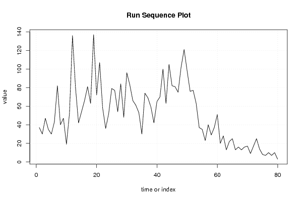
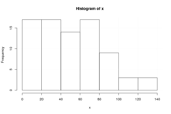
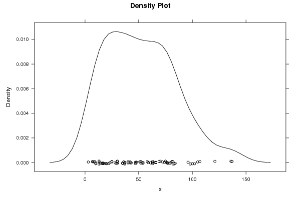
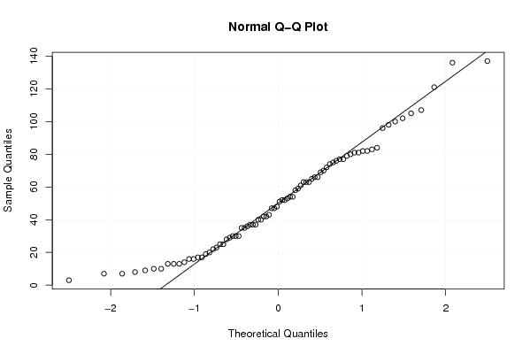
| Title produced by software | Univariate Explorative Data Analysis | ||||||||||||||||||||||||||||||||||||||||||||||||||||
| Date of computation | Tue, 02 Nov 2010 12:07:39 +0000 | ||||||||||||||||||||||||||||||||||||||||||||||||||||
| Cite this page as follows | Statistical Computations at FreeStatistics.org, Office for Research Development and Education, URL https://freestatistics.org/blog/index.php?v=date/2010/Nov/02/t1288699624lmcgi5o6s7m41zi.htm/, Retrieved Fri, 29 May 2026 18:29:24 +0000 | ||||||||||||||||||||||||||||||||||||||||||||||||||||
| Statistical Computations at FreeStatistics.org, Office for Research Development and Education, URL https://freestatistics.org/blog/index.php?pk=91291, Retrieved Fri, 29 May 2026 18:29:24 +0000 | |||||||||||||||||||||||||||||||||||||||||||||||||||||
| QR Codes: | |||||||||||||||||||||||||||||||||||||||||||||||||||||
|
| |||||||||||||||||||||||||||||||||||||||||||||||||||||
| Original text written by user: | |||||||||||||||||||||||||||||||||||||||||||||||||||||
| IsPrivate? | No (this computation is public) | ||||||||||||||||||||||||||||||||||||||||||||||||||||
| User-defined keywords | |||||||||||||||||||||||||||||||||||||||||||||||||||||
| Estimated Impact | 1251 | ||||||||||||||||||||||||||||||||||||||||||||||||||||
Tree of Dependent Computations | |||||||||||||||||||||||||||||||||||||||||||||||||||||
| Family? (F = Feedback message, R = changed R code, M = changed R Module, P = changed Parameters, D = changed Data) | |||||||||||||||||||||||||||||||||||||||||||||||||||||
| - [Univariate Explorative Data Analysis] [Monthly US soldie...] [2010-11-02 12:07:39] [d76b387543b13b5e3afd8ff9e5fdc89f] [Current] - RMP [(Partial) Autocorrelation Function] [Soldiers] [2010-11-29 09:48:36] [b98453cac15ba1066b407e146608df68] - PD [(Partial) Autocorrelation Function] [] [2010-12-03 11:32:19] [8a9a6f7c332640af31ddca253a8ded58] - PD [(Partial) Autocorrelation Function] [] [2010-12-03 14:12:17] [8a9a6f7c332640af31ddca253a8ded58] - PD [(Partial) Autocorrelation Function] [] [2010-12-03 14:14:33] [8a9a6f7c332640af31ddca253a8ded58] - D [(Partial) Autocorrelation Function] [] [2010-12-07 13:28:58] [f72e5115d7374b3b3f29ba3966e5379d] - P [(Partial) Autocorrelation Function] [] [2010-12-07 15:13:37] [f72e5115d7374b3b3f29ba3966e5379d] - P [(Partial) Autocorrelation Function] [] [2010-12-07 15:20:07] [f72e5115d7374b3b3f29ba3966e5379d] - RMP [Variance Reduction Matrix] [] [2010-12-07 15:29:14] [f72e5115d7374b3b3f29ba3966e5379d] - RMP [Standard Deviation-Mean Plot] [] [2010-12-07 15:39:58] [f72e5115d7374b3b3f29ba3966e5379d] - RMP [Spectral Analysis] [] [2010-12-07 16:29:36] [f72e5115d7374b3b3f29ba3966e5379d] - RMP [Spectral Analysis] [] [2010-12-07 16:34:30] [f72e5115d7374b3b3f29ba3966e5379d] - P [(Partial) Autocorrelation Function] [] [2010-12-17 14:07:41] [8a9a6f7c332640af31ddca253a8ded58] - P [(Partial) Autocorrelation Function] [] [2010-12-17 14:09:32] [8a9a6f7c332640af31ddca253a8ded58] - P [(Partial) Autocorrelation Function] [] [2010-12-17 14:11:00] [8a9a6f7c332640af31ddca253a8ded58] - PD [(Partial) Autocorrelation Function] [] [2010-12-14 12:47:55] [9b13650c94c5192ca5135ec8a1fa39f7] - PD [(Partial) Autocorrelation Function] [Workshop 9] [2010-12-14 12:34:06] [20c5a34fea7ed3b9b27ff444f2eb4dfe] - [(Partial) Autocorrelation Function] [Workshop 9] [2010-12-14 13:09:27] [20c5a34fea7ed3b9b27ff444f2eb4dfe] - R P [(Partial) Autocorrelation Function] [] [2011-01-10 20:58:25] [a7c91bc614e4e21e8b9c8593f39a36f1] - R PD [(Partial) Autocorrelation Function] [WS9_autocorrelation] [2011-12-06 18:22:15] [2adcc8dcd741502b8a9375c7fd3d7ce3] - RMPD [Spectral Analysis] [WS9_spectral-anal...] [2011-12-06 18:23:40] [2adcc8dcd741502b8a9375c7fd3d7ce3] - RM [Spectral Analysis] [P AF] [2011-12-17 17:18:03] [9ef609fa6add02911e58c08267119249] - RMPD [Variance Reduction Matrix] [WS9_variance-redu...] [2011-12-06 18:25:03] [2adcc8dcd741502b8a9375c7fd3d7ce3] - RM [Variance Reduction Matrix] [VRM] [2011-12-17 17:23:33] [9ef609fa6add02911e58c08267119249] - R P [(Partial) Autocorrelation Function] [Soldiers autocorr...] [2012-12-01 14:17:53] [22a7ed72f77de7f3efc5689ed05063a7] - R P [(Partial) Autocorrelation Function] [Soldiers] [2012-12-01 14:22:50] [22a7ed72f77de7f3efc5689ed05063a7] - P [(Partial) Autocorrelation Function] [Soldiers] [2012-12-01 14:26:54] [22a7ed72f77de7f3efc5689ed05063a7] - RMP [Spectral Analysis] [Soldiers] [2012-12-01 14:31:07] [22a7ed72f77de7f3efc5689ed05063a7] - RMP [Variance Reduction Matrix] [Soldiers VRM] [2012-12-01 14:39:07] [22a7ed72f77de7f3efc5689ed05063a7] - R P [(Partial) Autocorrelation Function] [] [2012-12-04 15:50:48] [74be16979710d4c4e7c6647856088456] - R P [(Partial) Autocorrelation Function] [] [2012-12-04 15:53:51] [74be16979710d4c4e7c6647856088456] - R P [(Partial) Autocorrelation Function] [paper arima acf] [2012-12-12 18:35:45] [74be16979710d4c4e7c6647856088456] - RMP [Spectral Analysis] [Soldiers] [2010-11-29 09:50:20] [b98453cac15ba1066b407e146608df68] - D [Spectral Analysis] [CP] [2010-12-04 08:37:02] [c1605865773cc027e55b238d879a644c] - R PD [Spectral Analysis] [] [2010-12-10 11:15:17] [22937c5b58c14f6c22964f32d64ff823] - PD [Spectral Analysis] [Cumulatief period...] [2010-12-12 14:28:13] [c1605865773cc027e55b238d879a644c] - D [Spectral Analysis] [ws 9] [2010-12-14 12:45:12] [20c5a34fea7ed3b9b27ff444f2eb4dfe] - P [Spectral Analysis] [ws 9] [2010-12-14 13:12:01] [20c5a34fea7ed3b9b27ff444f2eb4dfe] - RM [Standard Deviation-Mean Plot] [] [2010-12-14 13:28:34] [20c5a34fea7ed3b9b27ff444f2eb4dfe] - RM [ARIMA Backward Selection] [] [2010-12-14 13:51:17] [20c5a34fea7ed3b9b27ff444f2eb4dfe] - R [Spectral Analysis] [WS 9 - Cumulatiev...] [2011-12-01 16:49:05] [6a3e51c0c7ab195427042dfaef1df5a0] - P [Spectral Analysis] [WS 9 - Cumulatiev...] [2011-12-01 16:54:15] [6a3e51c0c7ab195427042dfaef1df5a0] - PD [Spectral Analysis] [Spectrum Analysis] [2011-12-07 13:53:52] [57eb71340681272e66d705d5c4d9e797] - RM [Spectral Analysis] [Spectrum analyses] [2011-12-21 13:00:05] [57eb71340681272e66d705d5c4d9e797] - RM [Spectral Analysis] [Spectrum analyses] [2011-12-21 13:00:05] [57eb71340681272e66d705d5c4d9e797] - R P [Spectral Analysis] [Spectrum analyses -] [2011-12-21 13:01:57] [57eb71340681272e66d705d5c4d9e797] - RMPD [Variance Reduction Matrix] [Variance Reductio...] [2011-12-07 13:59:45] [57eb71340681272e66d705d5c4d9e797] - R P [Variance Reduction Matrix] [Variance Reductio...] [2011-12-21 13:09:12] [57eb71340681272e66d705d5c4d9e797] - R P [Spectral Analysis] [PR CP Diff.] [2011-12-14 15:43:50] [b8fde34a99ee6a7d49500940cae4da2a] [Truncated] | |||||||||||||||||||||||||||||||||||||||||||||||||||||
| Feedback Forum | |||||||||||||||||||||||||||||||||||||||||||||||||||||
Post a new message | |||||||||||||||||||||||||||||||||||||||||||||||||||||
Dataset | |||||||||||||||||||||||||||||||||||||||||||||||||||||
| Dataseries X: | |||||||||||||||||||||||||||||||||||||||||||||||||||||
37 30 47 35 30 43 82 40 47 19 52 136 80 42 54 66 81 63 137 72 107 58 36 52 79 77 54 84 48 96 83 66 61 53 30 74 69 59 42 65 70 100 63 105 82 81 75 102 121 98 76 77 63 37 35 23 40 29 37 51 20 28 13 22 25 13 16 13 16 17 9 17 25 14 8 7 10 7 10 3 | |||||||||||||||||||||||||||||||||||||||||||||||||||||
Tables (Output of Computation) | |||||||||||||||||||||||||||||||||||||||||||||||||||||
| |||||||||||||||||||||||||||||||||||||||||||||||||||||
Figures (Output of Computation) | |||||||||||||||||||||||||||||||||||||||||||||||||||||
Input Parameters & R Code | |||||||||||||||||||||||||||||||||||||||||||||||||||||
| Parameters (Session): | |||||||||||||||||||||||||||||||||||||||||||||||||||||
| par1 = 8 ; par2 = 11 ; par3 = TRUE ; | |||||||||||||||||||||||||||||||||||||||||||||||||||||
| Parameters (R input): | |||||||||||||||||||||||||||||||||||||||||||||||||||||
| par1 = 0 ; par2 = 36 ; | |||||||||||||||||||||||||||||||||||||||||||||||||||||
| R code (references can be found in the software module): | |||||||||||||||||||||||||||||||||||||||||||||||||||||
par1 <- as.numeric(par1) | |||||||||||||||||||||||||||||||||||||||||||||||||||||