Repository of Reproducible Computations

Free Statistics

of Irreproducible Research!

Author's title

Author

*The author of this computation has been verified*

R Software Module

rwasp_autocorrelation.wasp

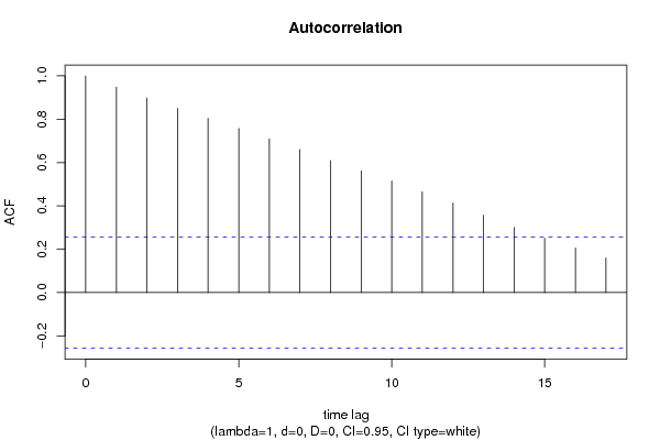
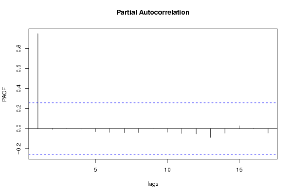
Title produced by software

(Partial) Autocorrelation Function

Date of computation

Fri, 03 Dec 2010 14:14:33 +0000

Cite this page as follows

Statistical Computations at FreeStatistics.org, Office for Research Development and Education, URL https://freestatistics.org/blog/index.php?v=date/2010/Dec/03/t1291385549ebhzyxplqht9szw.htm/, Retrieved Mon, 29 Apr 2024 06:42:50 +0000

Statistical Computations at FreeStatistics.org, Office for Research Development and Education, URL https://freestatistics.org/blog/index.php?pk=104815, Retrieved Mon, 29 Apr 2024 06:42:50 +0000

QR Codes:

Paste this QR Code to cite your computation.

Original text written by user:

IsPrivate?

No (this computation is public)

User-defined keywords

Estimated Impact

189

Family? (F = Feedback message, R = changed R code, M = changed R Module, P = changed Parameters, D = changed Data)

-     [Univariate Explorative Data Analysis] [Monthly US soldie...] [2010-11-02 12:07:39] [b98453cac15ba1066b407e146608df68]
- RMP   [(Partial) Autocorrelation Function] [Soldiers] [2010-11-29 09:48:36] [b98453cac15ba1066b407e146608df68]
-   PD    [(Partial) Autocorrelation Function] [] [2010-12-03 11:32:19] [8a9a6f7c332640af31ddca253a8ded58]
-   PD        [(Partial) Autocorrelation Function] [] [2010-12-03 14:14:33] [df17410ebb98883e83037e1662207ccb] [Current]
-    D          [(Partial) Autocorrelation Function] [] [2010-12-07 13:28:58] [f72e5115d7374b3b3f29ba3966e5379d] 
-   P             [(Partial) Autocorrelation Function] [] [2010-12-07 15:13:37] [f72e5115d7374b3b3f29ba3966e5379d] 
-   P             [(Partial) Autocorrelation Function] [] [2010-12-07 15:20:07] [f72e5115d7374b3b3f29ba3966e5379d] 
- RMP             [Variance Reduction Matrix] [] [2010-12-07 15:29:14] [f72e5115d7374b3b3f29ba3966e5379d] 
- RMP             [Standard Deviation-Mean Plot] [] [2010-12-07 15:39:58] [f72e5115d7374b3b3f29ba3966e5379d] 
- RMP             [Spectral Analysis] [] [2010-12-07 16:29:36] [f72e5115d7374b3b3f29ba3966e5379d] 
- RMP             [Spectral Analysis] [] [2010-12-07 16:34:30] [f72e5115d7374b3b3f29ba3966e5379d] 
-   P           [(Partial) Autocorrelation Function] [] [2010-12-17 14:07:41] [8a9a6f7c332640af31ddca253a8ded58] 
-   P           [(Partial) Autocorrelation Function] [] [2010-12-17 14:09:32] [8a9a6f7c332640af31ddca253a8ded58] 
-   P           [(Partial) Autocorrelation Function] [] [2010-12-17 14:11:00] [8a9a6f7c332640af31ddca253a8ded58] 

Feedback Forum

Post a new message

Dataseries X:

Download CSV

Histogram

Boxplots

Summary of computational transaction
Raw Input	view raw input (R code)
Raw Output	view raw output of R engine
Computing time	3 seconds
R Server	'George Udny Yule' @ 72.249.76.132

\begin{tabular}{lllllllll}
\hline
Summary of computational transaction \tabularnewline
Raw Input & view raw input (R code)  \tabularnewline
Raw Output & view raw output of R engine  \tabularnewline
Computing time & 3 seconds \tabularnewline
R Server & 'George Udny Yule' @ 72.249.76.132 \tabularnewline
\hline
\end{tabular}
%Source: https://freestatistics.org/blog/index.php?pk=104815&T=0

[TABLE]
[ROW][C]Summary of computational transaction[/C][/ROW]
[ROW][C]Raw Input[/C][C]view raw input (R code) [/C][/ROW]
[ROW][C]Raw Output[/C][C]view raw output of R engine [/C][/ROW]
[ROW][C]Computing time[/C][C]3 seconds[/C][/ROW]
[ROW][C]R Server[/C][C]'George Udny Yule' @ 72.249.76.132[/C][/ROW]
[/TABLE]
Source: https://freestatistics.org/blog/index.php?pk=104815&T=0

Globally Unique Identifier (entire table): ba.freestatistics.org/blog/index.php?pk=104815&T=0

As an alternative you can also use a QR Code:

The GUIDs for individual cells are displayed in the table below:

Summary of computational transaction
Raw Input	view raw input (R code)
Raw Output	view raw output of R engine
Computing time	3 seconds
R Server	'George Udny Yule' @ 72.249.76.132

Autocorrelation Function
Time lag k	ACF(k)	T-STAT	P-value
1	0.947992	7.2197	0
2	0.897972	6.8388	0
3	0.850458	6.4769	0
4	0.804251	6.125	0
5	0.757289	5.7673	0
6	0.709171	5.4009	1e-06
7	0.65971	5.0242	3e-06
8	0.609283	4.6402	1e-05
9	0.562341	4.2827	3.5e-05
10	0.514704	3.9199	0.000118
11	0.465169	3.5426	0.000395
12	0.413588	3.1498	0.001291
13	0.35691	2.7181	0.004322
14	0.300266	2.2868	0.012939
15	0.251156	1.9127	0.030361
16	0.205953	1.5685	0.061103
17	0.159246	1.2128	0.115065

\begin{tabular}{lllllllll}
\hline
Autocorrelation Function \tabularnewline
Time lag k & ACF(k) & T-STAT & P-value \tabularnewline
1 & 0.947992 & 7.2197 & 0 \tabularnewline
2 & 0.897972 & 6.8388 & 0 \tabularnewline
3 & 0.850458 & 6.4769 & 0 \tabularnewline
4 & 0.804251 & 6.125 & 0 \tabularnewline
5 & 0.757289 & 5.7673 & 0 \tabularnewline
6 & 0.709171 & 5.4009 & 1e-06 \tabularnewline
7 & 0.65971 & 5.0242 & 3e-06 \tabularnewline
8 & 0.609283 & 4.6402 & 1e-05 \tabularnewline
9 & 0.562341 & 4.2827 & 3.5e-05 \tabularnewline
10 & 0.514704 & 3.9199 & 0.000118 \tabularnewline
11 & 0.465169 & 3.5426 & 0.000395 \tabularnewline
12 & 0.413588 & 3.1498 & 0.001291 \tabularnewline
13 & 0.35691 & 2.7181 & 0.004322 \tabularnewline
14 & 0.300266 & 2.2868 & 0.012939 \tabularnewline
15 & 0.251156 & 1.9127 & 0.030361 \tabularnewline
16 & 0.205953 & 1.5685 & 0.061103 \tabularnewline
17 & 0.159246 & 1.2128 & 0.115065 \tabularnewline
\hline
\end{tabular}
%Source: https://freestatistics.org/blog/index.php?pk=104815&T=1

[TABLE]
[ROW][C]Autocorrelation Function[/C][/ROW]
[ROW][C]Time lag k[/C][C]ACF(k)[/C][C]T-STAT[/C][C]P-value[/C][/ROW]
[ROW][C]1[/C][C]0.947992[/C][C]7.2197[/C][C]0[/C][/ROW]
[ROW][C]2[/C][C]0.897972[/C][C]6.8388[/C][C]0[/C][/ROW]
[ROW][C]3[/C][C]0.850458[/C][C]6.4769[/C][C]0[/C][/ROW]
[ROW][C]4[/C][C]0.804251[/C][C]6.125[/C][C]0[/C][/ROW]
[ROW][C]5[/C][C]0.757289[/C][C]5.7673[/C][C]0[/C][/ROW]
[ROW][C]6[/C][C]0.709171[/C][C]5.4009[/C][C]1e-06[/C][/ROW]
[ROW][C]7[/C][C]0.65971[/C][C]5.0242[/C][C]3e-06[/C][/ROW]
[ROW][C]8[/C][C]0.609283[/C][C]4.6402[/C][C]1e-05[/C][/ROW]
[ROW][C]9[/C][C]0.562341[/C][C]4.2827[/C][C]3.5e-05[/C][/ROW]
[ROW][C]10[/C][C]0.514704[/C][C]3.9199[/C][C]0.000118[/C][/ROW]
[ROW][C]11[/C][C]0.465169[/C][C]3.5426[/C][C]0.000395[/C][/ROW]
[ROW][C]12[/C][C]0.413588[/C][C]3.1498[/C][C]0.001291[/C][/ROW]
[ROW][C]13[/C][C]0.35691[/C][C]2.7181[/C][C]0.004322[/C][/ROW]
[ROW][C]14[/C][C]0.300266[/C][C]2.2868[/C][C]0.012939[/C][/ROW]
[ROW][C]15[/C][C]0.251156[/C][C]1.9127[/C][C]0.030361[/C][/ROW]
[ROW][C]16[/C][C]0.205953[/C][C]1.5685[/C][C]0.061103[/C][/ROW]
[ROW][C]17[/C][C]0.159246[/C][C]1.2128[/C][C]0.115065[/C][/ROW]
[/TABLE]
Source: https://freestatistics.org/blog/index.php?pk=104815&T=1

Globally Unique Identifier (entire table): ba.freestatistics.org/blog/index.php?pk=104815&T=1

As an alternative you can also use a QR Code:

The GUIDs for individual cells are displayed in the table below:

Autocorrelation Function
Time lag k	ACF(k)	T-STAT	P-value
1	0.947992	7.2197	0
2	0.897972	6.8388	0
3	0.850458	6.4769	0
4	0.804251	6.125	0
5	0.757289	5.7673	0
6	0.709171	5.4009	1e-06
7	0.65971	5.0242	3e-06
8	0.609283	4.6402	1e-05
9	0.562341	4.2827	3.5e-05
10	0.514704	3.9199	0.000118
11	0.465169	3.5426	0.000395
12	0.413588	3.1498	0.001291
13	0.35691	2.7181	0.004322
14	0.300266	2.2868	0.012939
15	0.251156	1.9127	0.030361
16	0.205953	1.5685	0.061103
17	0.159246	1.2128	0.115065

Partial Autocorrelation Function
Time lag k	PACF(k)	T-STAT	P-value
1	0.947992	7.2197	0
2	-0.007077	-0.0539	0.478602
3	-0.001265	-0.0096	0.496174
4	-0.011893	-0.0906	0.46407
5	-0.032036	-0.244	0.404054
6	-0.037786	-0.2878	0.387275
7	-0.041985	-0.3197	0.375155
8	-0.040554	-0.3089	0.37927
9	0.001995	0.0152	0.493964
10	-0.036448	-0.2776	0.391161
11	-0.048973	-0.373	0.355265
12	-0.053883	-0.4104	0.341527
13	-0.089241	-0.6796	0.249719
14	-0.045585	-0.3472	0.364863
15	0.028485	0.2169	0.414511
16	0.001594	0.0121	0.495178
17	-0.045287	-0.3449	0.365709

\begin{tabular}{lllllllll}
\hline
Partial Autocorrelation Function \tabularnewline
Time lag k & PACF(k) & T-STAT & P-value \tabularnewline
1 & 0.947992 & 7.2197 & 0 \tabularnewline
2 & -0.007077 & -0.0539 & 0.478602 \tabularnewline
3 & -0.001265 & -0.0096 & 0.496174 \tabularnewline
4 & -0.011893 & -0.0906 & 0.46407 \tabularnewline
5 & -0.032036 & -0.244 & 0.404054 \tabularnewline
6 & -0.037786 & -0.2878 & 0.387275 \tabularnewline
7 & -0.041985 & -0.3197 & 0.375155 \tabularnewline
8 & -0.040554 & -0.3089 & 0.37927 \tabularnewline
9 & 0.001995 & 0.0152 & 0.493964 \tabularnewline
10 & -0.036448 & -0.2776 & 0.391161 \tabularnewline
11 & -0.048973 & -0.373 & 0.355265 \tabularnewline
12 & -0.053883 & -0.4104 & 0.341527 \tabularnewline
13 & -0.089241 & -0.6796 & 0.249719 \tabularnewline
14 & -0.045585 & -0.3472 & 0.364863 \tabularnewline
15 & 0.028485 & 0.2169 & 0.414511 \tabularnewline
16 & 0.001594 & 0.0121 & 0.495178 \tabularnewline
17 & -0.045287 & -0.3449 & 0.365709 \tabularnewline
\hline
\end{tabular}
%Source: https://freestatistics.org/blog/index.php?pk=104815&T=2

[TABLE]
[ROW][C]Partial Autocorrelation Function[/C][/ROW]
[ROW][C]Time lag k[/C][C]PACF(k)[/C][C]T-STAT[/C][C]P-value[/C][/ROW]
[ROW][C]1[/C][C]0.947992[/C][C]7.2197[/C][C]0[/C][/ROW]
[ROW][C]2[/C][C]-0.007077[/C][C]-0.0539[/C][C]0.478602[/C][/ROW]
[ROW][C]3[/C][C]-0.001265[/C][C]-0.0096[/C][C]0.496174[/C][/ROW]
[ROW][C]4[/C][C]-0.011893[/C][C]-0.0906[/C][C]0.46407[/C][/ROW]
[ROW][C]5[/C][C]-0.032036[/C][C]-0.244[/C][C]0.404054[/C][/ROW]
[ROW][C]6[/C][C]-0.037786[/C][C]-0.2878[/C][C]0.387275[/C][/ROW]
[ROW][C]7[/C][C]-0.041985[/C][C]-0.3197[/C][C]0.375155[/C][/ROW]
[ROW][C]8[/C][C]-0.040554[/C][C]-0.3089[/C][C]0.37927[/C][/ROW]
[ROW][C]9[/C][C]0.001995[/C][C]0.0152[/C][C]0.493964[/C][/ROW]
[ROW][C]10[/C][C]-0.036448[/C][C]-0.2776[/C][C]0.391161[/C][/ROW]
[ROW][C]11[/C][C]-0.048973[/C][C]-0.373[/C][C]0.355265[/C][/ROW]
[ROW][C]12[/C][C]-0.053883[/C][C]-0.4104[/C][C]0.341527[/C][/ROW]
[ROW][C]13[/C][C]-0.089241[/C][C]-0.6796[/C][C]0.249719[/C][/ROW]
[ROW][C]14[/C][C]-0.045585[/C][C]-0.3472[/C][C]0.364863[/C][/ROW]
[ROW][C]15[/C][C]0.028485[/C][C]0.2169[/C][C]0.414511[/C][/ROW]
[ROW][C]16[/C][C]0.001594[/C][C]0.0121[/C][C]0.495178[/C][/ROW]
[ROW][C]17[/C][C]-0.045287[/C][C]-0.3449[/C][C]0.365709[/C][/ROW]
[/TABLE]
Source: https://freestatistics.org/blog/index.php?pk=104815&T=2

Globally Unique Identifier (entire table): ba.freestatistics.org/blog/index.php?pk=104815&T=2

As an alternative you can also use a QR Code:

The GUIDs for individual cells are displayed in the table below:

Partial Autocorrelation Function
Time lag k	PACF(k)	T-STAT	P-value
1	0.947992	7.2197	0
2	-0.007077	-0.0539	0.478602
3	-0.001265	-0.0096	0.496174
4	-0.011893	-0.0906	0.46407
5	-0.032036	-0.244	0.404054
6	-0.037786	-0.2878	0.387275
7	-0.041985	-0.3197	0.375155
8	-0.040554	-0.3089	0.37927
9	0.001995	0.0152	0.493964
10	-0.036448	-0.2776	0.391161
11	-0.048973	-0.373	0.355265
12	-0.053883	-0.4104	0.341527
13	-0.089241	-0.6796	0.249719
14	-0.045585	-0.3472	0.364863
15	0.028485	0.2169	0.414511
16	0.001594	0.0121	0.495178
17	-0.045287	-0.3449	0.365709

Figure 1

PNG link

Postscript link

PDF link

Figure 2

PNG link

Postscript link

PDF link

Parameters (Session):

par1 = Default ; par2 = 1 ; par3 = 0 ; par4 = 0 ; par5 = 12 ; par6 = White Noise ; par7 = 0.95 ;

Parameters (R input):

par1 = Default ; par2 = 1 ; par3 = 0 ; par4 = 0 ; par5 = 12 ; par6 = White Noise ; par7 = 0.95 ;

R code (references can be found in the software module):

if (par1 == 'Default') {
par1 = 10*log10(length(x))
} else {
par1 <- as.numeric(par1)
}
par2 <- as.numeric(par2)
par3 <- as.numeric(par3)
par4 <- as.numeric(par4)
par5 <- as.numeric(par5)
if (par6 == 'White Noise') par6 <- 'white' else par6 <- 'ma'
par7 <- as.numeric(par7)
if (par2 == 0) {
x <- log(x)
} else {
x <- (x ^ par2 - 1) / par2
}
if (par3 > 0) x <- diff(x,lag=1,difference=par3)
if (par4 > 0) x <- diff(x,lag=par5,difference=par4)
bitmap(file='pic1.png')
racf <- acf(x, par1, main='Autocorrelation', xlab='time lag', ylab='ACF', ci.type=par6, ci=par7, sub=paste('(lambda=',par2,', d=',par3,', D=',par4,', CI=', par7, ', CI type=',par6,')',sep=''))
dev.off()
bitmap(file='pic2.png')
rpacf <- pacf(x,par1,main='Partial Autocorrelation',xlab='lags',ylab='PACF')
dev.off()
(myacf <- c(racf$acf))
(mypacf <- c(rpacf$acf))
lengthx <- length(x)
sqrtn <- sqrt(lengthx)
load(file='createtable')
a<-table.start()
a<-table.row.start(a)
a<-table.element(a,'Autocorrelation Function',4,TRUE)
a<-table.row.end(a)
a<-table.row.start(a)
a<-table.element(a,'Time lag k',header=TRUE)
a<-table.element(a,hyperlink('basics.htm','ACF(k)','click here for more information about the Autocorrelation Function'),header=TRUE)
a<-table.element(a,'T-STAT',header=TRUE)
a<-table.element(a,'P-value',header=TRUE)
a<-table.row.end(a)
for (i in 2:(par1+1)) {
a<-table.row.start(a)
a<-table.element(a,i-1,header=TRUE)
a<-table.element(a,round(myacf[i],6))
mytstat <- myacf[i]*sqrtn
a<-table.element(a,round(mytstat,4))
a<-table.element(a,round(1-pt(abs(mytstat),lengthx),6))
a<-table.row.end(a)
}
a<-table.end(a)
table.save(a,file='mytable.tab')
a<-table.start()
a<-table.row.start(a)
a<-table.element(a,'Partial Autocorrelation Function',4,TRUE)
a<-table.row.end(a)
a<-table.row.start(a)
a<-table.element(a,'Time lag k',header=TRUE)
a<-table.element(a,hyperlink('basics.htm','PACF(k)','click here for more information about the Partial Autocorrelation Function'),header=TRUE)
a<-table.element(a,'T-STAT',header=TRUE)
a<-table.element(a,'P-value',header=TRUE)
a<-table.row.end(a)
for (i in 1:par1) {
a<-table.row.start(a)
a<-table.element(a,i,header=TRUE)
a<-table.element(a,round(mypacf[i],6))
mytstat <- mypacf[i]*sqrtn
a<-table.element(a,round(mytstat,4))
a<-table.element(a,round(1-pt(abs(mytstat),lengthx),6))
a<-table.row.end(a)
}
a<-table.end(a)
table.save(a,file='mytable1.tab')

Free Statistics

Description of Statistical Computation

Tree of Dependent Computations

Dataset

Tables (Output of Computation)

Figures (Output of Computation)

Input Parameters & R Code