Free Statistics
of Irreproducible Research!
Description of Statistical Computation | |||||||||||||||||||||||||||||||||||||||||||||||||||||||||||||||||||||||||||||||||||||||||||||||||||||||||||||
|---|---|---|---|---|---|---|---|---|---|---|---|---|---|---|---|---|---|---|---|---|---|---|---|---|---|---|---|---|---|---|---|---|---|---|---|---|---|---|---|---|---|---|---|---|---|---|---|---|---|---|---|---|---|---|---|---|---|---|---|---|---|---|---|---|---|---|---|---|---|---|---|---|---|---|---|---|---|---|---|---|---|---|---|---|---|---|---|---|---|---|---|---|---|---|---|---|---|---|---|---|---|---|---|---|---|---|---|---|---|
| Author's title | |||||||||||||||||||||||||||||||||||||||||||||||||||||||||||||||||||||||||||||||||||||||||||||||||||||||||||||
| Author | *The author of this computation has been verified* | ||||||||||||||||||||||||||||||||||||||||||||||||||||||||||||||||||||||||||||||||||||||||||||||||||||||||||||
| R Software Module | rwasp_correlation.wasp | ||||||||||||||||||||||||||||||||||||||||||||||||||||||||||||||||||||||||||||||||||||||||||||||||||||||||||||
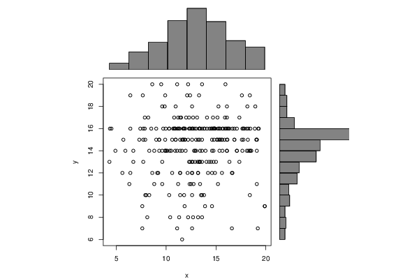
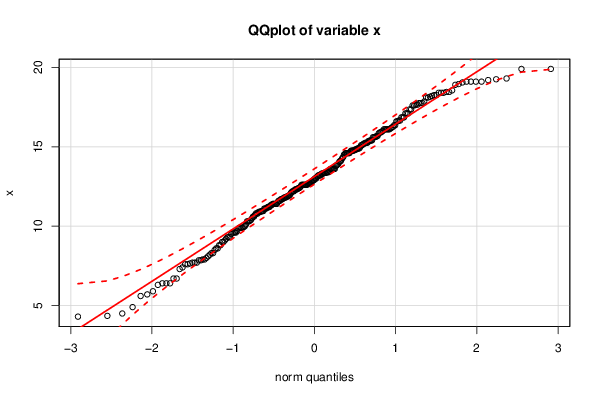
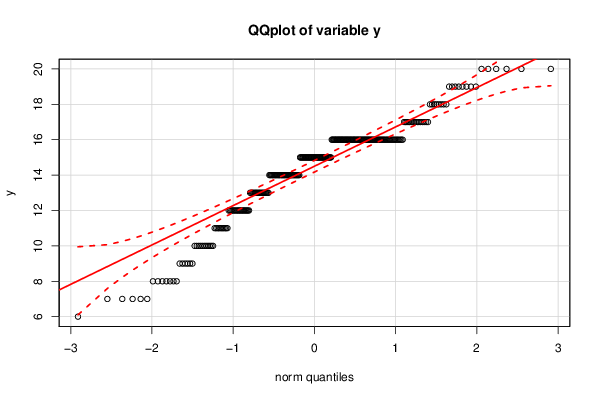
| Title produced by software | Pearson Correlation | ||||||||||||||||||||||||||||||||||||||||||||||||||||||||||||||||||||||||||||||||||||||||||||||||||||||||||||
| Date of computation | Wed, 17 Dec 2014 09:36:47 +0000 | ||||||||||||||||||||||||||||||||||||||||||||||||||||||||||||||||||||||||||||||||||||||||||||||||||||||||||||
| Cite this page as follows | Statistical Computations at FreeStatistics.org, Office for Research Development and Education, URL https://freestatistics.org/blog/index.php?v=date/2014/Dec/17/t1418809047dfcctmzyz3o4ewd.htm/, Retrieved Sat, 02 May 2026 18:36:35 +0000 | ||||||||||||||||||||||||||||||||||||||||||||||||||||||||||||||||||||||||||||||||||||||||||||||||||||||||||||
| Statistical Computations at FreeStatistics.org, Office for Research Development and Education, URL https://freestatistics.org/blog/index.php?pk=270006, Retrieved Sat, 02 May 2026 18:36:35 +0000 | |||||||||||||||||||||||||||||||||||||||||||||||||||||||||||||||||||||||||||||||||||||||||||||||||||||||||||||
| QR Codes: | |||||||||||||||||||||||||||||||||||||||||||||||||||||||||||||||||||||||||||||||||||||||||||||||||||||||||||||
|
| |||||||||||||||||||||||||||||||||||||||||||||||||||||||||||||||||||||||||||||||||||||||||||||||||||||||||||||
| Original text written by user: | |||||||||||||||||||||||||||||||||||||||||||||||||||||||||||||||||||||||||||||||||||||||||||||||||||||||||||||
| IsPrivate? | No (this computation is public) | ||||||||||||||||||||||||||||||||||||||||||||||||||||||||||||||||||||||||||||||||||||||||||||||||||||||||||||
| User-defined keywords | |||||||||||||||||||||||||||||||||||||||||||||||||||||||||||||||||||||||||||||||||||||||||||||||||||||||||||||
| Estimated Impact | 495 | ||||||||||||||||||||||||||||||||||||||||||||||||||||||||||||||||||||||||||||||||||||||||||||||||||||||||||||
Tree of Dependent Computations | |||||||||||||||||||||||||||||||||||||||||||||||||||||||||||||||||||||||||||||||||||||||||||||||||||||||||||||
| Family? (F = Feedback message, R = changed R code, M = changed R Module, P = changed Parameters, D = changed Data) | |||||||||||||||||||||||||||||||||||||||||||||||||||||||||||||||||||||||||||||||||||||||||||||||||||||||||||||
| F [Histogram] [Frequency Plot (C...] [2010-09-25 09:09:15] [b98453cac15ba1066b407e146608df68] - D [Histogram] [Market Share of O...] [2010-10-04 13:35:10] [b98453cac15ba1066b407e146608df68] - RMPD [Histogram] [bachelor of schak...] [2014-12-16 12:24:13] [9378e2688aa9dcfd1390615d31e9d404] - RMPD [Pearson Correlation] [] [2014-12-17 09:29:37] [2b9d0c54c8c845c625e475ed5f1f3af1] - R D [Pearson Correlation] [] [2014-12-17 09:36:47] [b22ed12f8980e34362f6926e9ebd1315] [Current] | |||||||||||||||||||||||||||||||||||||||||||||||||||||||||||||||||||||||||||||||||||||||||||||||||||||||||||||
| Feedback Forum | |||||||||||||||||||||||||||||||||||||||||||||||||||||||||||||||||||||||||||||||||||||||||||||||||||||||||||||
Post a new message | |||||||||||||||||||||||||||||||||||||||||||||||||||||||||||||||||||||||||||||||||||||||||||||||||||||||||||||
Dataset | |||||||||||||||||||||||||||||||||||||||||||||||||||||||||||||||||||||||||||||||||||||||||||||||||||||||||||||
| Dataseries X: | |||||||||||||||||||||||||||||||||||||||||||||||||||||||||||||||||||||||||||||||||||||||||||||||||||||||||||||
12,9 12,2 12,8 7,4 6,7 12,6 14,8 13,3 11,1 8,2 11,4 6,4 10,6 12,0 6,3 11,3 11,9 9,3 9,6 10,0 6,4 13,8 10,8 13,8 11,7 10,9 16,1 13,4 9,9 11,5 8,3 11,7 9,0 9,7 10,8 10,3 10,4 12,7 9,3 11,8 5,9 11,4 13,0 10,8 12,3 11,3 11,8 7,9 12,7 12,3 11,6 6,7 10,9 12,1 13,3 10,1 5,7 14,3 8,0 13,3 9,3 12,5 7,6 15,9 9,2 9,1 11,1 13,0 14,5 12,2 12,3 11,4 8,8 14,6 12,6 13,0 12,6 13,2 9,9 7,7 10,5 13,4 10,9 4,3 10,3 11,8 11,2 11,4 8,6 13,2 12,6 5,6 9,9 8,8 7,7 9,0 7,3 11,4 13,6 7,9 10,7 10,3 8,3 9,6 14,2 8,5 13,5 4,9 6,4 9,6 11,6 11,1 4,35 12,7 18,1 17,85 16,6 12,6 17,1 19,1 16,1 13,35 18,4 14,7 10,6 12,6 16,2 13,6 18,9 14,1 14,5 16,15 14,75 14,8 12,45 12,65 17,35 8,6 18,4 16,1 11,6 17,75 15,25 17,65 16,35 17,65 13,6 14,35 14,75 18,25 9,9 16 18,25 16,85 14,6 13,85 18,95 15,6 14,85 11,75 18,45 15,9 17,1 16,1 19,9 10,95 18,45 15,1 15 11,35 15,95 18,1 14,6 15,4 15,4 17,6 13,35 19,1 15,35 7,6 13,4 13,9 19,1 15,25 12,9 16,1 17,35 13,15 12,15 12,6 10,35 15,4 9,6 18,2 13,6 14,85 14,75 14,1 14,9 16,25 19,25 13,6 13,6 15,65 12,75 14,6 9,85 12,65 19,2 16,6 11,2 15,25 11,9 13,2 16,35 12,4 15,85 18,15 11,15 15,65 17,75 7,65 12,35 15,6 19,3 15,2 17,1 15,6 18,4 19,05 18,55 19,1 13,1 12,85 9,5 4,5 11,85 13,6 11,7 12,4 13,35 11,4 14,9 19,9 11,2 14,6 17,6 14,05 16,1 13,35 11,85 11,95 14,75 15,15 13,2 16,85 7,85 7,7 12,6 7,85 10,95 12,35 9,95 14,9 16,65 13,4 13,95 15,7 16,85 10,95 15,35 12,2 15,1 17,75 15,2 14,6 16,65 8,1 | |||||||||||||||||||||||||||||||||||||||||||||||||||||||||||||||||||||||||||||||||||||||||||||||||||||||||||||
| Dataseries Y: | |||||||||||||||||||||||||||||||||||||||||||||||||||||||||||||||||||||||||||||||||||||||||||||||||||||||||||||
13 8 14 16 14 13 15 13 20 17 15 16 12 17 11 16 16 15 13 14 19 16 17 10 15 14 14 16 15 17 14 16 15 16 16 10 8 17 14 10 14 12 16 16 16 8 16 15 8 13 14 13 16 19 19 14 15 13 10 16 15 11 9 16 12 12 14 14 13 15 17 14 11 9 7 15 12 15 14 16 14 13 16 13 16 16 16 10 12 12 12 12 19 14 13 16 15 12 8 10 16 16 10 18 12 16 10 14 12 11 15 7 16 16 16 16 12 15 14 15 16 13 10 17 15 18 16 20 16 17 16 15 13 16 16 16 17 20 14 17 6 16 15 16 16 14 16 16 16 14 14 16 16 15 16 16 18 15 16 16 16 17 14 18 9 15 14 15 13 16 20 14 12 15 15 15 16 11 16 7 11 9 15 16 14 15 13 13 12 16 14 16 14 15 10 16 14 16 12 16 16 15 14 16 11 15 18 13 7 7 17 18 15 8 13 13 15 18 16 14 15 19 16 12 16 11 16 15 19 15 14 14 17 16 20 16 9 13 15 19 16 17 16 9 11 14 19 13 14 15 15 14 16 17 12 15 17 15 10 16 15 11 16 16 16 14 14 16 16 18 14 20 15 16 16 16 12 8 | |||||||||||||||||||||||||||||||||||||||||||||||||||||||||||||||||||||||||||||||||||||||||||||||||||||||||||||
Tables (Output of Computation) | |||||||||||||||||||||||||||||||||||||||||||||||||||||||||||||||||||||||||||||||||||||||||||||||||||||||||||||
| |||||||||||||||||||||||||||||||||||||||||||||||||||||||||||||||||||||||||||||||||||||||||||||||||||||||||||||
Figures (Output of Computation) | |||||||||||||||||||||||||||||||||||||||||||||||||||||||||||||||||||||||||||||||||||||||||||||||||||||||||||||
Input Parameters & R Code | |||||||||||||||||||||||||||||||||||||||||||||||||||||||||||||||||||||||||||||||||||||||||||||||||||||||||||||
| Parameters (Session): | |||||||||||||||||||||||||||||||||||||||||||||||||||||||||||||||||||||||||||||||||||||||||||||||||||||||||||||
| Parameters (R input): | |||||||||||||||||||||||||||||||||||||||||||||||||||||||||||||||||||||||||||||||||||||||||||||||||||||||||||||
| R code (references can be found in the software module): | |||||||||||||||||||||||||||||||||||||||||||||||||||||||||||||||||||||||||||||||||||||||||||||||||||||||||||||
x <- x[!is.na(y)] | |||||||||||||||||||||||||||||||||||||||||||||||||||||||||||||||||||||||||||||||||||||||||||||||||||||||||||||