Repository of Reproducible Computations

Free Statistics

of Irreproducible Research!

Author's title

Author

*The author of this computation has been verified*

R Software Module

Ian.Hollidayrwasp_Reddy-Moores Data Boxplot V2.0.wasp

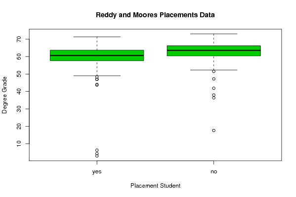
Title produced by software

Boxplot and Trimmed Means

Date of computation

Wed, 13 Oct 2010 09:46:26 +0000

Cite this page as follows

Statistical Computations at FreeStatistics.org, Office for Research Development and Education, URL https://freestatistics.org/blog/index.php?v=date/2010/Oct/13/t1286963135awxk4ye3ncncuo5.htm/, Retrieved Sun, 28 Apr 2024 16:52:24 +0000

Statistical Computations at FreeStatistics.org, Office for Research Development and Education, URL https://freestatistics.org/blog/index.php?pk=83079, Retrieved Sun, 28 Apr 2024 16:52:24 +0000

QR Codes:

Paste this QR Code to cite your computation.

Original text written by user:

IsPrivate?

No (this computation is public)

User-defined keywords

Reddy Moores (2006) Placement data

Estimated Impact

394

Family? (F = Feedback message, R = changed R code, M = changed R Module, P = changed Parameters, D = changed Data)

-     [Boxplot and Trimmed Means] [Reddy Moores Boxp...] [2010-10-12 16:37:57] [98fd0e87c3eb04e0cc2efde01dbafab6]
- R P     [Boxplot and Trimmed Means] [Reddy-Moores Plac...] [2010-10-13 09:46:26] [a9208f4f8d3b118336aae915785f2bd9] [Current]
-   P       [Boxplot and Trimmed Means] [Boxplot 5%] [2010-10-13 15:21:51] [571c005f5a0ec004107e098ce4a713be] 
-   P         [Boxplot and Trimmed Means] [Boxplot 10%  ] [2010-10-13 15:27:26] [571c005f5a0ec004107e098ce4a713be] 
-   P           [Boxplot and Trimmed Means] [Boxplot 20%] [2010-10-13 15:32:56] [571c005f5a0ec004107e098ce4a713be] 
-    D      [Boxplot and Trimmed Means] [Compendium week 2] [2010-10-14 11:34:06] [e41d04f9b27258a4b30e5e5545051fd7] 
-    D      [Boxplot and Trimmed Means] [c2 no] [2010-10-14 11:39:21] [e41d04f9b27258a4b30e5e5545051fd7] 
-           [Boxplot and Trimmed Means] [] [2010-10-14 11:41:02] [74be16979710d4c4e7c6647856088456] 
-             [Boxplot and Trimmed Means] [] [2010-10-14 11:45:00] [74be16979710d4c4e7c6647856088456] 
-    D      [Boxplot and Trimmed Means] [] [2010-10-14 11:52:25] [74be16979710d4c4e7c6647856088456] 
-           [Boxplot and Trimmed Means] [] [2010-10-14 12:41:52] [b48f5f730c5d512b3990977e77ceb182] 
-    D      [Boxplot and Trimmed Means] [Boxplot] [2010-10-14 17:35:07] [88bba52b01540967ecde38774018061d] 
-    D      [Boxplot and Trimmed Means] [boxplot] [2010-10-14 17:48:02] [88bba52b01540967ecde38774018061d] 
-    D      [Boxplot and Trimmed Means] [boxplot] [2010-10-14 18:24:00] [88bba52b01540967ecde38774018061d] 
-    D      [Boxplot and Trimmed Means] [boxplot] [2010-10-14 18:32:31] [88bba52b01540967ecde38774018061d] 
- R P       [Boxplot and Trimmed Means] [Boxplot error = n...] [2010-10-15 11:04:33] [98fd0e87c3eb04e0cc2efde01dbafab6] 
- RMPD      [Notched Boxplots] [] [2010-10-15 11:13:23] [b98453cac15ba1066b407e146608df68] 
-             [Notched Boxplots] [Workshop 3: Quest...] [2010-10-23 09:08:24] [62f7c80c4d96454bbd2b2b026ea9aad9] 
- RMPD        [Chi-Squared and McNemar Tests] [] [2010-11-09 09:02:39] [8a9a6f7c332640af31ddca253a8ded58] 
-    D          [Chi-Squared and McNemar Tests] [] [2010-11-09 09:07:32] [8a9a6f7c332640af31ddca253a8ded58] 
-    D            [Chi-Squared and McNemar Tests] [] [2010-11-09 09:11:59] [8a9a6f7c332640af31ddca253a8ded58] 
-    D              [Chi-Squared and McNemar Tests] [] [2010-11-09 09:13:25] [8a9a6f7c332640af31ddca253a8ded58] 
-    D              [Chi-Squared and McNemar Tests] [] [2010-11-09 09:14:37] [8a9a6f7c332640af31ddca253a8ded58] 
-    D              [Chi-Squared and McNemar Tests] [] [2010-11-09 09:16:01] [8a9a6f7c332640af31ddca253a8ded58] 
-    D              [Chi-Squared and McNemar Tests] [] [2010-11-09 09:17:45] [8a9a6f7c332640af31ddca253a8ded58] 
-    D                [Chi-Squared and McNemar Tests] [] [2010-11-09 09:24:50] [8a9a6f7c332640af31ddca253a8ded58] 
- R           [Notched Boxplots] [Workshop 4 questi...] [2011-10-12 15:00:44] [3346191a817a30d0b56421a47a7031a4] 
- RMPD        [Minimum Sample Size - Testing Mean] [Workshop 4 questi...] [2011-10-12 15:08:12] [3346191a817a30d0b56421a47a7031a4] 
- RMPD        [Testing Mean with unknown Variance - Critical Value] [] [2011-10-12 18:06:55] [2adcc8dcd741502b8a9375c7fd3d7ce3] 
- R           [Notched Boxplots] [] [2011-10-20 11:15:25] [80bca13c5f9401fbb753952fd2952f4a] 
-  M            [Notched Boxplots] [] [2011-10-20 11:25:00] [80bca13c5f9401fbb753952fd2952f4a] 
- R           [Notched Boxplots] [] [2011-10-20 11:27:37] [19d77e37efa419fdc040c74a96874aff] 
- R  D        [Notched Boxplots] [Treatment E] [2011-10-20 12:52:57] [380049693c521f4999989215fb37aeca] 
- R  D        [Notched Boxplots] [Treatment S] [2011-10-20 13:05:50] [380049693c521f4999989215fb37aeca] 
- R  D        [Notched Boxplots] [Treatment T] [2011-10-20 13:07:50] [380049693c521f4999989215fb37aeca] 
- R  D        [Notched Boxplots] [] [2011-10-21 20:00:09] [1dc3906a3b5a6ec06dc921f387100c9e] 
-    D          [Notched Boxplots] [] [2011-10-21 20:04:22] [1dc3906a3b5a6ec06dc921f387100c9e] 
-    D            [Notched Boxplots] [] [2011-10-21 20:06:21] [1dc3906a3b5a6ec06dc921f387100c9e] 
- RMPD        [Minimum Sample Size - Testing Mean] [] [2011-10-24 12:59:57] [a1957df0bc37aec4aa3c994e6a08412c] 
- R P           [Minimum Sample Size - Testing Mean] [] [2011-10-25 17:14:21] [a1957df0bc37aec4aa3c994e6a08412c] 
- RMPD        [Minimum Sample Size - Testing Mean] [] [2011-10-25 11:15:33] [86a47bcc75cd2e0d5b5c9888edc893c2] 
- R           [Notched Boxplots] [] [2011-10-25 18:39:07] [19d77e37efa419fdc040c74a96874aff] 
- R           [Notched Boxplots] [] [2011-11-08 21:51:36] [46d7ccc24e5d35a2decd922dfb3b3a39] 
- R           [Notched Boxplots] [] [2011-12-14 10:41:57] [59e8d6f9dbd0564968d0bb4af7b45de5] 
- R  D        [Notched Boxplots] [] [2011-12-16 13:19:22] [8fcdd1f5b88bf5ac5d2a0b8a91219b89] 
- RM          [Notched Boxplots] [] [2011-12-21 12:19:53] [98f3ba974ec9d6d754dcc83206539a91] 
- R           [Notched Boxplots] [] [2011-12-23 11:21:47] [a9671b130b33f9fcb98554992ce4582f] 
- R  D        [Notched Boxplots] [] [2011-12-23 11:36:04] [a9671b130b33f9fcb98554992ce4582f] 
- RMPD        [Testing Mean with unknown Variance - Critical Value] [WS4 - question 4] [2012-10-08 14:49:02] [fe055a25191a04e375a94ef97fddf389] 
- RMPD        [Testing Mean with unknown Variance - Critical Value] [WS4_Q2_H3] [2012-10-08 20:22:51] [be6dd99035eed41c2358246baf91f928] 

[Truncated]

Feedback Forum

Post a new message

Dataseries X:

Download CSV

Histogram

Boxplots

'yes'	70.80
'yes'	69.60
'yes'	69.87
'yes'	67.47
'yes'	67.60
'yes'	67.13
'yes'	66.27
'yes'	66.73
'yes'	68.07
'yes'	67.80
'yes'	64.80
'yes'	64.60
'yes'	64.20
'yes'	64.20
'yes'	63.67
'yes'	61.00
'yes'	59.67
'yes'	59.67
'yes'	59.80
'yes'	60.73
'yes'	59.40
'yes'	58.07
'yes'	57.47
'yes'	70.73
'yes'	72.87
'yes'	66.00
'yes'	66.07
'yes'	66.00
'yes'	66.27
'yes'	64.00
'yes'	63.67
'yes'	63.73
'yes'	63.33
'yes'	63.53
'yes'	63.53
'yes'	62.87
'yes'	59.53
'yes'	62.80
'yes'	60.80
'yes'	59.80
'yes'	56.67
'yes'	57.67
'yes'	58.40
'yes'	55.47
'yes'	56.20
'yes'	71.53
'yes'	68.67
'yes'	65.67
'yes'	66.73
'yes'	67.33
'yes'	66.73
'yes'	66.87
'yes'	65.80
'yes'	64.73
'yes'	65.47
'yes'	63.60
'yes'	64.07
'yes'	64.67
'yes'	63.73
'yes'	62.53
'yes'	61.93
'yes'	62.67
'yes'	62.80
'yes'	61.33
'yes'	62.60
'yes'	59.13
'yes'	61.27
'yes'	59.47
'yes'	57.87
'yes'	59.73
'yes'	61.40
'yes'	58.80
'yes'	58.33
'yes'	57.47
'yes'	57.13
'yes'	55.00
'yes'	51.53
'yes'	72.73
'yes'	73.00
'yes'	70.80
'yes'	70.07
'yes'	71.67
'yes'	71.07
'yes'	70.67
'yes'	70.73
'yes'	70.73
'yes'	68.60
'yes'	69.60
'yes'	66.47
'yes'	67.07
'yes'	68.67
'yes'	66.93
'yes'	65.93
'yes'	68.87
'yes'	66.53
'yes'	65.80
'yes'	66.60
'yes'	66.00
'yes'	65.00
'yes'	66.80
'yes'	65.60
'yes'	66.00
'yes'	65.67
'yes'	64.67
'yes'	65.07
'yes'	64.67
'yes'	65.07
'yes'	65.20
'yes'	64.87
'yes'	63.47
'yes'	62.60
'yes'	64.07
'yes'	63.73
'yes'	64.67
'yes'	61.60
'yes'	61.60
'yes'	60.47
'yes'	61.27
'yes'	63.00
'yes'	61.47
'yes'	60.87
'yes'	61.67
'yes'	62.87
'yes'	62.40
'yes'	59.73
'yes'	60.13
'yes'	58.80
'yes'	59.60
'yes'	58.93
'yes'	60.13
'yes'	58.20
'yes'	58.27
'yes'	58.27
'yes'	55.07
'yes'	53.87
'yes'	52.33
'yes'	47.20
'yes'	37.93
'yes'	72.73
'yes'	70.07
'yes'	70.67
'yes'	72.07
'yes'	68.80
'yes'	68.80
'yes'	67.47
'yes'	66.73
'yes'	66.53
'yes'	66.00
'yes'	67.60
'yes'	66.00
'yes'	66.00
'yes'	66.53
'yes'	65.80
'yes'	64.27
'yes'	64.67
'yes'	64.60
'yes'	64.13
'yes'	65.47
'yes'	62.93
'yes'	63.53
'yes'	62.13
'yes'	63.87
'yes'	64.67
'yes'	63.33
'yes'	63.13
'yes'	62.80
'yes'	62.40
'yes'	62.40
'yes'	62.60
'yes'	61.47
'yes'	62.20
'yes'	63.00
'yes'	61.80
'yes'	59.73
'yes'	60.33
'yes'	60.13
'yes'	59.53
'yes'	59.00
'yes'	55.93
'yes'	41.87
'yes'	36.33
'yes'	71.67
'yes'	71.47
'yes'	70.47
'yes'	69.53
'yes'	70.73
'yes'	69.93
'yes'	68.73
'yes'	67.53
'yes'	64.40
'yes'	66.20
'yes'	66.20
'yes'	63.07
'yes'	64.27
'yes'	65.00
'yes'	63.67
'yes'	62.67
'yes'	64.67
'yes'	64.67
'yes'	64.47
'yes'	61.93
'yes'	63.27
'yes'	62.93
'yes'	61.93
'yes'	64.07
'yes'	61.40
'yes'	62.00
'yes'	62.60
'yes'	62.40
'yes'	61.60
'yes'	59.87
'yes'	63.20
'yes'	62.40
'yes'	60.40
'yes'	61.87
'yes'	59.13
'yes'	59.53
'yes'	57.80
'yes'	57.67
'yes'	61.00
'yes'	56.33
'yes'	54.20
'yes'	54.73
'yes'	52.67
'yes'	17.60
'no'	66.67
'no'	66.33
'no'	64.33
'no'	64.00
'no'	63.33
'no'	61.33
'no'	64.67
'no'	63.00
'no'	60.67
'no'	63.67
'no'	60.67
'no'	61.67
'no'	62.33
'no'	60.33
'no'	59.67
'no'	60.33
'no'	59.33
'no'	58.67
'no'	58.67
'no'	59.33
'no'	57.33
'no'	59.33
'no'	56.00
'no'	53.67
'no'	58.67
'no'	49.33
'no'	71.33
'no'	70.33
'no'	69.00
'no'	66.00
'no'	66.00
'no'	63.33
'no'	65.33
'no'	64.33
'no'	64.00
'no'	61.67
'no'	63.67
'no'	64.67
'no'	61.67
'no'	62.00
'no'	61.33
'no'	63.67
'no'	61.33
'no'	62.33
'no'	59.67
'no'	59.33
'no'	61.67
'no'	58.67
'no'	58.00
'no'	56.67
'no'	59.67
'no'	58.00
'no'	57.00
'no'	57.67
'no'	58.67
'no'	55.33
'no'	56.00
'no'	55.67
'no'	53.33
'no'	53.67
'no'	51.00
'no'	47.00
'no'	4.33
'no'	70.00
'no'	68.67
'no'	67.67
'no'	66.00
'no'	65.67
'no'	65.67
'no'	63.67
'no'	63.67
'no'	64.00
'no'	62.00
'no'	62.00
'no'	61.67
'no'	61.67
'no'	63.33
'no'	61.00
'no'	62.33
'no'	60.33
'no'	60.33
'no'	60.67
'no'	57.67
'no'	58.33
'no'	58.00
'no'	57.33
'no'	56.67
'no'	58.00
'no'	55.33
'no'	55.67
'no'	54.67
'no'	56.33
'no'	55.00
'no'	55.00
'no'	54.67
'no'	54.33
'no'	49.00
'no'	48.33
'no'	49.67
'no'	43.67
'no'	6.33
'no'	3.00
'no'	66.67
'no'	67.33
'no'	65.33
'no'	66.00
'no'	65.67
'no'	66.67
'no'	65.67
'no'	65.00
'no'	64.67
'no'	66.67
'no'	63.67
'no'	63.33
'no'	63.67
'no'	63.33
'no'	63.67
'no'	63.00
'no'	61.67
'no'	61.33
'no'	60.67
'no'	60.00
'no'	61.67
'no'	61.33
'no'	58.67
'no'	60.33
'no'	59.67
'no'	59.33
'no'	59.67
'no'	61.00
'no'	61.00
'no'	60.00
'no'	60.00
'no'	58.67
'no'	58.33
'no'	58.00
'no'	56.33
'no'	54.67
'no'	55.33
'no'	54.00
'no'	52.67
'no'	44.00
'no'	65.67
'no'	65.00
'no'	66.33
'no'	64.00
'no'	62.33
'no'	61.33
'no'	63.00
'no'	63.67
'no'	62.00
'no'	61.33
'no'	64.67
'no'	62.67
'no'	64.00
'no'	61.00
'no'	60.67
'no'	59.67
'no'	60.33
'no'	56.67
'no'	56.67
'no'	54.33
'no'	51.00
'no'	51.00
'no'	47.00
'no'	68.00
'no'	65.00
'no'	64.00
'no'	64.00
'no'	64.00
'no'	62.00
'no'	61.00
'no'	60.00
'no'	60.00
'no'	62.00
'no'	60.00
'no'	59.00
'no'	61.00
'no'	60.00
'no'	60.00
'no'	58.00
'no'	58.00
'no'	60.00
'no'	58.00
'no'	59.00
'no'	56.00
'no'	54.00
'no'	51.00
'no'	47.00

Summary of computational transaction
Raw Input	view raw input (R code)
Raw Output	view raw output of R engine
Computing time	1 seconds
R Server	'George Udny Yule' @ 72.249.76.132

\begin{tabular}{lllllllll}
\hline
Summary of computational transaction \tabularnewline
Raw Input & view raw input (R code)  \tabularnewline
Raw Output & view raw output of R engine  \tabularnewline
Computing time & 1 seconds \tabularnewline
R Server & 'George Udny Yule' @ 72.249.76.132 \tabularnewline
\hline
\end{tabular}
%Source: https://freestatistics.org/blog/index.php?pk=83079&T=0

[TABLE]
[ROW][C]Summary of computational transaction[/C][/ROW]
[ROW][C]Raw Input[/C][C]view raw input (R code) [/C][/ROW]
[ROW][C]Raw Output[/C][C]view raw output of R engine [/C][/ROW]
[ROW][C]Computing time[/C][C]1 seconds[/C][/ROW]
[ROW][C]R Server[/C][C]'George Udny Yule' @ 72.249.76.132[/C][/ROW]
[/TABLE]
Source: https://freestatistics.org/blog/index.php?pk=83079&T=0

Globally Unique Identifier (entire table): ba.freestatistics.org/blog/index.php?pk=83079&T=0

As an alternative you can also use a QR Code:

The GUIDs for individual cells are displayed in the table below:

Summary of computational transaction
Raw Input	view raw input (R code)
Raw Output	view raw output of R engine
Computing time	1 seconds
R Server	'George Udny Yule' @ 72.249.76.132

Boxplot statistics
Placement	lower whisker	lower hinge	median	upper hinge	upper whisker
yes	49	57.67	60.67	63.67	71.33
no	52.33	60.47	63.6	66.27	73

\begin{tabular}{lllllllll}
\hline
Boxplot statistics \tabularnewline
Placement & lower whisker & lower hinge & median & upper hinge & upper whisker \tabularnewline
yes & 49 & 57.67 & 60.67 & 63.67 & 71.33 \tabularnewline
no & 52.33 & 60.47 & 63.6 & 66.27 & 73 \tabularnewline
\hline
\end{tabular}
%Source: https://freestatistics.org/blog/index.php?pk=83079&T=1

[TABLE]
[ROW][C]Boxplot statistics[/C][/ROW]
[ROW][C]Placement[/C][C]lower whisker[/C][C]lower hinge[/C][C]median[/C][C]upper hinge[/C][C]upper whisker[/C][/ROW]
[ROW][C]yes[/C][C]49[/C][C]57.67[/C][C]60.67[/C][C]63.67[/C][C]71.33[/C][/ROW]
[ROW][C]no[/C][C]52.33[/C][C]60.47[/C][C]63.6[/C][C]66.27[/C][C]73[/C][/ROW]
[/TABLE]
Source: https://freestatistics.org/blog/index.php?pk=83079&T=1

Globally Unique Identifier (entire table): ba.freestatistics.org/blog/index.php?pk=83079&T=1

As an alternative you can also use a QR Code:

The GUIDs for individual cells are displayed in the table below:

Boxplot statistics
Placement	lower whisker	lower hinge	median	upper hinge	upper whisker
yes	49	57.67	60.67	63.67	71.33
no	52.33	60.47	63.6	66.27	73

Trimmed Mean Equation
Placement	No Placement
59.3018518518519	63.0598222222222

\begin{tabular}{lllllllll}
\hline
Trimmed Mean Equation \tabularnewline
Placement & No Placement \tabularnewline
59.3018518518519 & 63.0598222222222 \tabularnewline
\hline
\end{tabular}
%Source: https://freestatistics.org/blog/index.php?pk=83079&T=2

[TABLE]
[ROW][C]Trimmed Mean Equation[/C][/ROW]
[ROW][C]Placement[/C][C]No Placement[/C][/ROW]
[ROW][C]59.3018518518519[/C][C]63.0598222222222[/C][/ROW]
[/TABLE]
Source: https://freestatistics.org/blog/index.php?pk=83079&T=2

Globally Unique Identifier (entire table): ba.freestatistics.org/blog/index.php?pk=83079&T=2

As an alternative you can also use a QR Code:

The GUIDs for individual cells are displayed in the table below:

Trimmed Mean Equation
Placement	No Placement
59.3018518518519	63.0598222222222

Figure 1

PNG link

Postscript link

PDF link

Parameters (Session):

par1 = 3 ; par2 = FALSE ; par3 = 0 ; par4 = 1 ; par5 = 2 ;

Parameters (R input):

par1 = 3 ; par2 = FALSE ; par3 = 0 ; par4 = 1 ; par5 = 2 ;

R code (references can be found in the software module):

par1 <- as.numeric(par1) # colour
par2<- as.logical(par2) # notches ?
par3<-as.numeric(par3) # % trim
if(par3>45){par3<-45;warning('trim limited to 45%')}
if(par3<0){par3<-0;warning('negative trim makes no sense. Trim is zero.')}
par4 <- as.numeric(par4) #factor column
par5 <- as.numeric(par5) # response column
x <- t(x)
x1<-as.numeric(x[,par5]) # response
f1<-as.character(x[,par4]) # factor
x2<-x1[f1=='yes']
f2 <- f1[f1=='yes']
lotrm<-as.integer(length(x2)*par3/100)
hitrm<-as.integer(length(x2)*(100-par3)/100)
srt<-order(x2,f2)
trmx1<-x2[srt[lotrm:hitrm]]
trmf1<-f2[srt[lotrm:hitrm]]
x3<-x1[f1=='no']
f3 <- f1[f1=='no']
lotrm<-as.integer(length(x3)*par3/100)
hitrm<-as.integer(length(x3)*(100-par3)/100)
srt<-order(x3,f3)
trmx2<-x3[srt[lotrm:hitrm]]
trmf2<-f3[srt[lotrm:hitrm]]
xtrm<-c(trmx1,trmx2)
ftrm<-c(trmf1,trmf2)
xtrm[1:6]
ftrm[1:6]
bitmap(file='test1.png')
r<-boxplot(xtrm~as.factor(ftrm), col=par1, notch=par2, names =c('yes', 'no'), main='Reddy and Moores Placements Data', xlab='Placement Student', ylab='Degree Grade')
dev.off()
load(file='createtable')
a<-table.start()
a<-table.row.start(a)
a<-table.element(a,hyperlink('overview.htm','Boxplot statistics','Boxplot overview'),6,TRUE)
a<-table.row.end(a)
a<-table.row.start(a)
a<-table.element(a,'Placement',1,TRUE)
a<-table.element(a,hyperlink('lower_whisker.htm','lower whisker','definition of lower whisker'),1,TRUE)
a<-table.element(a,hyperlink('lower_hinge.htm','lower hinge','definition of lower hinge'),1,TRUE)
a<-table.element(a,hyperlink('central_tendency.htm','median','definitions about measures of central tendency'),1,TRUE)
a<-table.element(a,hyperlink('upper_hinge.htm','upper hinge','definition of upper hinge'),1,TRUE)
a<-table.element(a,hyperlink('upper_whisker.htm','upper whisker','definition of upper whisker'),1,TRUE)
a<-table.row.end(a)
a<-table.row.start(a)
a<-table.element(a,'yes',1,TRUE)
for (j in 1:5)
{
a<-table.element(a,r$stats[j,1])
}
a<-table.row.end(a)
a<-table.row.start(a)
a<-table.element(a,'no',1,TRUE)
for (j in 1:5)
{
a<-table.element(a,r$stats[j,2])
}
a<-table.row.end(a)
a<-table.end(a)
table.save(a,file='mytable.tab')
tr.mns<-tapply(x1,f1,mean, trim=par3/100)
a<-table.start()
a<-table.row.start(a)
a<-table.element(a,hyperlink('trimmed_mean.htm','Trimmed Mean Equation','Trimmed Mean'),2,TRUE)
a<-table.row.end(a)
a<-table.row.start(a)
a<-table.element(a,'Placement')
a<-table.element(a,'No Placement')
a<-table.row.end(a)
a<-table.row.start(a)
a<-table.element(a,tr.mns[1])
a<-table.element(a,tr.mns[2])
a<-table.row.end(a)
a<-table.end(a)
table.save(a,file='mytable1.tab')

Free Statistics

Description of Statistical Computation

Tree of Dependent Computations

Dataset

Tables (Output of Computation)

Figures (Output of Computation)

Input Parameters & R Code