Free Statistics
of Irreproducible Research!
Description of Statistical Computation | |||||||||||||||||||||||||||||||||||||||||||||||||||||||||||||
|---|---|---|---|---|---|---|---|---|---|---|---|---|---|---|---|---|---|---|---|---|---|---|---|---|---|---|---|---|---|---|---|---|---|---|---|---|---|---|---|---|---|---|---|---|---|---|---|---|---|---|---|---|---|---|---|---|---|---|---|---|---|
| Author's title | |||||||||||||||||||||||||||||||||||||||||||||||||||||||||||||
| Author | *The author of this computation has been verified* | ||||||||||||||||||||||||||||||||||||||||||||||||||||||||||||
| R Software Module | rwasp_linear_regression.wasp | ||||||||||||||||||||||||||||||||||||||||||||||||||||||||||||
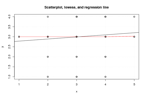
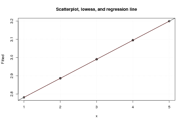
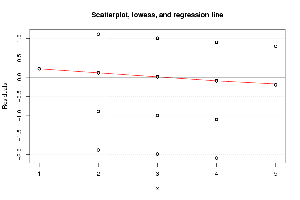
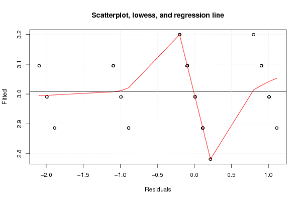
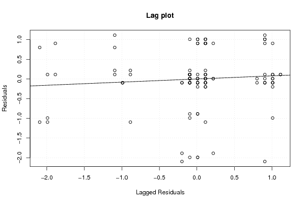
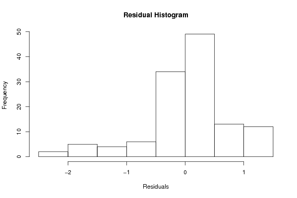
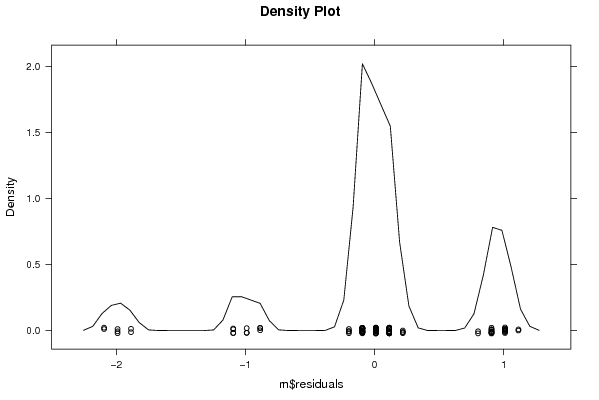
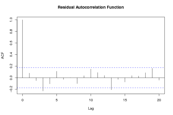
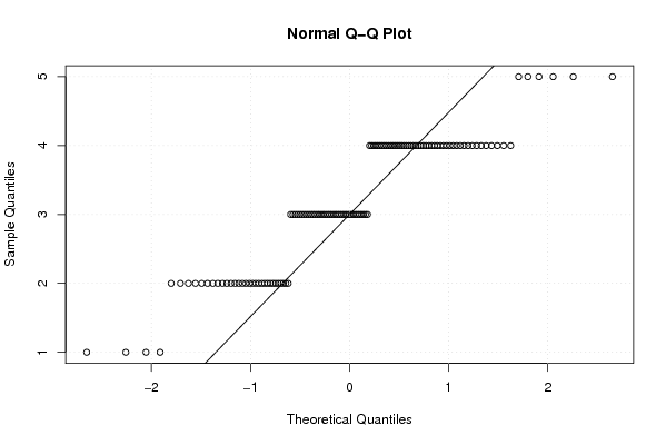
| Title produced by software | Linear Regression Graphical Model Validation | ||||||||||||||||||||||||||||||||||||||||||||||||||||||||||||
| Date of computation | Sat, 13 Nov 2010 11:31:05 +0000 | ||||||||||||||||||||||||||||||||||||||||||||||||||||||||||||
| Cite this page as follows | Statistical Computations at FreeStatistics.org, Office for Research Development and Education, URL https://freestatistics.org/blog/index.php?v=date/2010/Nov/13/t12896523062524dwm3hz276x2.htm/, Retrieved Mon, 01 Jun 2026 01:50:18 +0000 | ||||||||||||||||||||||||||||||||||||||||||||||||||||||||||||
| Statistical Computations at FreeStatistics.org, Office for Research Development and Education, URL https://freestatistics.org/blog/index.php?pk=94361, Retrieved Mon, 01 Jun 2026 01:50:18 +0000 | |||||||||||||||||||||||||||||||||||||||||||||||||||||||||||||
| QR Codes: | |||||||||||||||||||||||||||||||||||||||||||||||||||||||||||||
|
| |||||||||||||||||||||||||||||||||||||||||||||||||||||||||||||
| Original text written by user: | |||||||||||||||||||||||||||||||||||||||||||||||||||||||||||||
| IsPrivate? | No (this computation is public) | ||||||||||||||||||||||||||||||||||||||||||||||||||||||||||||
| User-defined keywords | |||||||||||||||||||||||||||||||||||||||||||||||||||||||||||||
| Estimated Impact | 558 | ||||||||||||||||||||||||||||||||||||||||||||||||||||||||||||
Tree of Dependent Computations | |||||||||||||||||||||||||||||||||||||||||||||||||||||||||||||
| Family? (F = Feedback message, R = changed R code, M = changed R Module, P = changed Parameters, D = changed Data) | |||||||||||||||||||||||||||||||||||||||||||||||||||||||||||||
| - [Linear Regression Graphical Model Validation] [Colombia Coffee -...] [2008-02-26 10:22:06] [74be16979710d4c4e7c6647856088456] - M D [Linear Regression Graphical Model Validation] [ws6vb] [2010-11-13 11:31:05] [0cadca125c925bcc9e6efbdd1941e458] [Current] - D [Linear Regression Graphical Model Validation] [tt] [2010-11-13 12:51:28] [4a7069087cf9e0eda253aeed7d8c30d6] - D [Linear Regression Graphical Model Validation] [W6tutorial] [2010-11-13 14:33:02] [c7506ced21a6c0dca45d37c8a93c80e0] - D [Linear Regression Graphical Model Validation] [Workshop 6, Mini ...] [2010-11-14 15:39:04] [3635fb7041b1998c5a1332cf9de22bce] - D [Linear Regression Graphical Model Validation] [Workshop 6, Simpl...] [2010-11-16 19:47:28] [3635fb7041b1998c5a1332cf9de22bce] - R D [Linear Regression Graphical Model Validation] [Mini Toturial - H...] [2010-11-17 00:22:02] [b20a509e36241371274681d9edf773da] - R D [Linear Regression Graphical Model Validation] [] [2011-11-15 15:55:49] [46896e8a404bb9354f2d070359621409] - R D [Linear Regression Graphical Model Validation] [Mini Tutorial - k...] [2011-11-15 16:56:43] [74be16979710d4c4e7c6647856088456] - RMPD [Chi-Squared Test, McNemar Test, and Fisher Exact Test] [Chi Squared Test ...] [2011-11-15 17:42:51] [d0cddc92c01af61bef0226b9e5ade9b3] - R D [Linear Regression Graphical Model Validation] [Mini Toturial - H...] [2010-11-17 00:19:55] [b20a509e36241371274681d9edf773da] - D [Linear Regression Graphical Model Validation] [] [2011-11-15 08:53:32] [ea9976aa04c7322b215e949114660791] - R D [Linear Regression Graphical Model Validation] [] [2011-11-15 15:35:27] [46896e8a404bb9354f2d070359621409] - R D [Linear Regression Graphical Model Validation] [Mini Tutorial - t...] [2011-11-15 16:42:35] [74be16979710d4c4e7c6647856088456] - R D [Linear Regression Graphical Model Validation] [Workshop 6: Mini-...] [2011-11-15 17:30:14] [21b3d52ef28595defb5676e0f3570994] - R D [Linear Regression Graphical Model Validation] [Workshop 6: Mini-...] [2011-11-15 17:32:29] [21b3d52ef28595defb5676e0f3570994] - R D [Linear Regression Graphical Model Validation] [] [2011-12-19 16:17:39] [c505444e07acba7694d29053ca5d114e] - R D [Linear Regression Graphical Model Validation] [] [2011-12-19 16:19:11] [c505444e07acba7694d29053ca5d114e] - [Linear Regression Graphical Model Validation] [Tutorial1] [2010-11-16 20:35:31] [fc9068db680cd880760a7c0fccd81a61] F D [Linear Regression Graphical Model Validation] [] [2010-11-17 08:28:03] [f9eaed74daea918f73b9f505c5b1f19e] - D [Linear Regression Graphical Model Validation] [Spaargeld NL vs L...] [2010-12-21 14:30:35] [fc9068db680cd880760a7c0fccd81a61] - D [Linear Regression Graphical Model Validation] [Spaargeld NL vs L...] [2010-12-21 14:42:24] [fc9068db680cd880760a7c0fccd81a61] | |||||||||||||||||||||||||||||||||||||||||||||||||||||||||||||
| Feedback Forum | |||||||||||||||||||||||||||||||||||||||||||||||||||||||||||||
Post a new message | |||||||||||||||||||||||||||||||||||||||||||||||||||||||||||||
Dataset | |||||||||||||||||||||||||||||||||||||||||||||||||||||||||||||
| Dataseries X: | |||||||||||||||||||||||||||||||||||||||||||||||||||||||||||||
4 3 5 4 2 4 3 2 4 2 4 2 5 3 4 3 4 2 3 4 2 4 4 3 4 2 4 4 4 2 4 4 4 4 3 4 3 3 3 2 4 4 4 3 4 4 3 1 4 4 2 2 4 3 1 4 2 4 5 3 2 4 2 2 2 4 5 4 5 2 3 4 3 2 3 4 1 2 2 3 3 2 2 4 3 3 4 4 2 2 4 3 2 4 3 3 4 4 3 3 3 2 2 1 2 3 3 3 3 4 2 3 3 4 3 3 3 4 4 3 4 5 2 4 3 | |||||||||||||||||||||||||||||||||||||||||||||||||||||||||||||
| Dataseries Y: | |||||||||||||||||||||||||||||||||||||||||||||||||||||||||||||
3 3 4 2 2 3 3 3 3 3 4 1 3 3 3 3 3 3 1 3 3 3 3 4 4 3 2 1 4 3 3 3 3 4 4 3 2 1 3 3 3 3 3 4 4 4 3 3 3 4 3 4 4 3 3 2 3 3 3 4 3 3 3 3 3 3 4 1 3 3 4 4 3 3 3 4 3 3 2 3 4 3 4 2 1 3 3 4 3 3 3 4 3 3 3 3 3 3 3 4 3 3 1 3 2 3 3 3 3 3 3 4 3 3 2 4 3 3 3 2 3 3 3 3 3 | |||||||||||||||||||||||||||||||||||||||||||||||||||||||||||||
Tables (Output of Computation) | |||||||||||||||||||||||||||||||||||||||||||||||||||||||||||||
| |||||||||||||||||||||||||||||||||||||||||||||||||||||||||||||
Figures (Output of Computation) | |||||||||||||||||||||||||||||||||||||||||||||||||||||||||||||
Input Parameters & R Code | |||||||||||||||||||||||||||||||||||||||||||||||||||||||||||||
| Parameters (Session): | |||||||||||||||||||||||||||||||||||||||||||||||||||||||||||||
| par1 = 0 ; | |||||||||||||||||||||||||||||||||||||||||||||||||||||||||||||
| Parameters (R input): | |||||||||||||||||||||||||||||||||||||||||||||||||||||||||||||
| par1 = 0 ; par2 = ; par3 = ; par4 = ; par5 = ; par6 = ; par7 = ; par8 = ; par9 = ; par10 = ; par11 = ; par12 = ; par13 = ; par14 = ; par15 = ; par16 = ; par17 = ; par18 = ; par19 = ; par20 = ; | |||||||||||||||||||||||||||||||||||||||||||||||||||||||||||||
| R code (references can be found in the software module): | |||||||||||||||||||||||||||||||||||||||||||||||||||||||||||||
par1 <- as.numeric(par1) | |||||||||||||||||||||||||||||||||||||||||||||||||||||||||||||