Free Statistics
of Irreproducible Research!
Description of Statistical Computation | |||||||||||||||||||||||||||||||||||||||||||||||||||||||||||||
|---|---|---|---|---|---|---|---|---|---|---|---|---|---|---|---|---|---|---|---|---|---|---|---|---|---|---|---|---|---|---|---|---|---|---|---|---|---|---|---|---|---|---|---|---|---|---|---|---|---|---|---|---|---|---|---|---|---|---|---|---|---|
| Author's title | |||||||||||||||||||||||||||||||||||||||||||||||||||||||||||||
| Author | *The author of this computation has been verified* | ||||||||||||||||||||||||||||||||||||||||||||||||||||||||||||
| R Software Module | rwasp_linear_regression.wasp | ||||||||||||||||||||||||||||||||||||||||||||||||||||||||||||
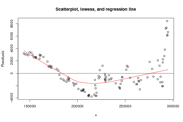
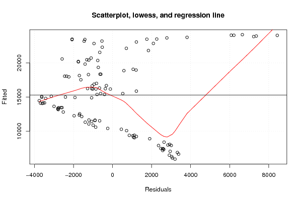
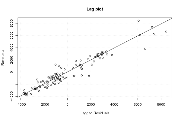
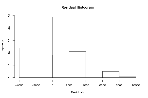
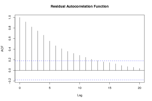
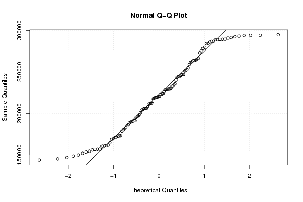
| Title produced by software | Linear Regression Graphical Model Validation | ||||||||||||||||||||||||||||||||||||||||||||||||||||||||||||
| Date of computation | Tue, 21 Dec 2010 14:42:24 +0000 | ||||||||||||||||||||||||||||||||||||||||||||||||||||||||||||
| Cite this page as follows | Statistical Computations at FreeStatistics.org, Office for Research Development and Education, URL https://freestatistics.org/blog/index.php?v=date/2010/Dec/21/t129294247661kdcqqrx0pa0v6.htm/, Retrieved Tue, 28 Jul 2026 16:23:20 +0000 | ||||||||||||||||||||||||||||||||||||||||||||||||||||||||||||
| Statistical Computations at FreeStatistics.org, Office for Research Development and Education, URL https://freestatistics.org/blog/index.php?pk=113627, Retrieved Tue, 28 Jul 2026 16:23:20 +0000 | |||||||||||||||||||||||||||||||||||||||||||||||||||||||||||||
| QR Codes: | |||||||||||||||||||||||||||||||||||||||||||||||||||||||||||||
|
| |||||||||||||||||||||||||||||||||||||||||||||||||||||||||||||
| Original text written by user: | |||||||||||||||||||||||||||||||||||||||||||||||||||||||||||||
| IsPrivate? | No (this computation is public) | ||||||||||||||||||||||||||||||||||||||||||||||||||||||||||||
| User-defined keywords | |||||||||||||||||||||||||||||||||||||||||||||||||||||||||||||
| Estimated Impact | 518 | ||||||||||||||||||||||||||||||||||||||||||||||||||||||||||||
Tree of Dependent Computations | |||||||||||||||||||||||||||||||||||||||||||||||||||||||||||||
| Family? (F = Feedback message, R = changed R code, M = changed R Module, P = changed Parameters, D = changed Data) | |||||||||||||||||||||||||||||||||||||||||||||||||||||||||||||
| - [Linear Regression Graphical Model Validation] [Colombia Coffee -...] [2008-02-26 10:22:06] [74be16979710d4c4e7c6647856088456] - M D [Linear Regression Graphical Model Validation] [ws6vb] [2010-11-13 11:31:05] [c7506ced21a6c0dca45d37c8a93c80e0] - D [Linear Regression Graphical Model Validation] [tt] [2010-11-13 12:51:28] [4a7069087cf9e0eda253aeed7d8c30d6] - D [Linear Regression Graphical Model Validation] [W6tutorial] [2010-11-13 14:33:02] [c7506ced21a6c0dca45d37c8a93c80e0] - D [Linear Regression Graphical Model Validation] [Spaargeld NL vs L...] [2010-12-21 14:42:24] [a8abc7260f3c847aeac0a796e7895a2e] [Current] | |||||||||||||||||||||||||||||||||||||||||||||||||||||||||||||
| Feedback Forum | |||||||||||||||||||||||||||||||||||||||||||||||||||||||||||||
Post a new message | |||||||||||||||||||||||||||||||||||||||||||||||||||||||||||||
Dataset | |||||||||||||||||||||||||||||||||||||||||||||||||||||||||||||
| Dataseries X: | |||||||||||||||||||||||||||||||||||||||||||||||||||||||||||||
143827 145191 146832 148577 149873 151847 153252 154292 155657 156523 156416 156693 160312 160438 160882 161668 164391 168556 169738 170387 171294 172202 172651 172770 178366 180014 181067 182586 184957 186417 188599 189490 190264 191221 191110 190674 195438 196393 197172 198760 200945 203845 204613 205487 206100 206315 206291 207801 211653 211325 211893 212056 214696 217455 218884 219816 219984 219062 218550 218179 222218 222196 223393 223292 226236 228831 228745 229140 229270 229359 230006 228810 232677 232961 234629 235660 240024 243554 244368 244356 245126 246321 246797 246735 251083 251786 252732 255051 259022 261698 263891 265247 262228 263429 264305 266371 273248 275472 278146 279506 283991 286794 288703 289285 288869 286942 285833 284095 289229 289389 290793 291454 294733 293853 294056 293982 293075 292391 | |||||||||||||||||||||||||||||||||||||||||||||||||||||||||||||
| Dataseries Y: | |||||||||||||||||||||||||||||||||||||||||||||||||||||||||||||
9113 9140 9309 9395 10027 10202 10003 9745 9966 10035 9999 9943 10258 10926 10807 10992 11034 10801 10161 10191 10451 10380 10251 10522 10801 10731 10161 9728 9882 9839 9917 10356 10857 10424 10721 10669 10565 10289 10646 10858 10282 10377 10443 10561 10668 10818 10865 10636 10409 10460 10579 10664 10711 11374 11345 11456 11966 12580 13006 13815 14579 14960 14904 16028 17079 15155 16049 15841 15159 14956 15645 15318 15595 16355 15925 16175 15900 15711 15594 15693 16438 17048 17699 17733 19439 20148 20112 18607 18409 18388 19187 17983 18449 19589 19135 19604 20877 23639 22830 21760 21879 21712 21321 21396 22000 22642 24272 24933 25219 25745 26433 27546 30774 32456 30124 30250 31288 31072 | |||||||||||||||||||||||||||||||||||||||||||||||||||||||||||||
Tables (Output of Computation) | |||||||||||||||||||||||||||||||||||||||||||||||||||||||||||||
| |||||||||||||||||||||||||||||||||||||||||||||||||||||||||||||
Figures (Output of Computation) | |||||||||||||||||||||||||||||||||||||||||||||||||||||||||||||
Input Parameters & R Code | |||||||||||||||||||||||||||||||||||||||||||||||||||||||||||||
| Parameters (Session): | |||||||||||||||||||||||||||||||||||||||||||||||||||||||||||||
| par1 = 0 ; | |||||||||||||||||||||||||||||||||||||||||||||||||||||||||||||
| Parameters (R input): | |||||||||||||||||||||||||||||||||||||||||||||||||||||||||||||
| par1 = 0 ; | |||||||||||||||||||||||||||||||||||||||||||||||||||||||||||||
| R code (references can be found in the software module): | |||||||||||||||||||||||||||||||||||||||||||||||||||||||||||||
par1 <- as.numeric(par1) | |||||||||||||||||||||||||||||||||||||||||||||||||||||||||||||