Free Statistics
of Irreproducible Research!
Description of Statistical Computation | |||||||||||||||||||||||||||||||||||||||||||||||||||||||||||||
|---|---|---|---|---|---|---|---|---|---|---|---|---|---|---|---|---|---|---|---|---|---|---|---|---|---|---|---|---|---|---|---|---|---|---|---|---|---|---|---|---|---|---|---|---|---|---|---|---|---|---|---|---|---|---|---|---|---|---|---|---|---|
| Author's title | |||||||||||||||||||||||||||||||||||||||||||||||||||||||||||||
| Author | *The author of this computation has been verified* | ||||||||||||||||||||||||||||||||||||||||||||||||||||||||||||
| R Software Module | rwasp_linear_regression.wasp | ||||||||||||||||||||||||||||||||||||||||||||||||||||||||||||
| Title produced by software | Linear Regression Graphical Model Validation | ||||||||||||||||||||||||||||||||||||||||||||||||||||||||||||
| Date of computation | Fri, 12 Nov 2010 11:48:01 +0000 | ||||||||||||||||||||||||||||||||||||||||||||||||||||||||||||
| Cite this page as follows | Statistical Computations at FreeStatistics.org, Office for Research Development and Education, URL https://freestatistics.org/blog/index.php?v=date/2010/Nov/12/t1289562463nqz9i8mrhcb5dd2.htm/, Retrieved Sun, 26 Oct 2025 13:47:30 +0000 | ||||||||||||||||||||||||||||||||||||||||||||||||||||||||||||
| Statistical Computations at FreeStatistics.org, Office for Research Development and Education, URL https://freestatistics.org/blog/index.php?pk=94100, Retrieved Sun, 26 Oct 2025 13:47:30 +0000 | |||||||||||||||||||||||||||||||||||||||||||||||||||||||||||||
| QR Codes: | |||||||||||||||||||||||||||||||||||||||||||||||||||||||||||||
|
| |||||||||||||||||||||||||||||||||||||||||||||||||||||||||||||
| Original text written by user: | |||||||||||||||||||||||||||||||||||||||||||||||||||||||||||||
| IsPrivate? | No (this computation is public) | ||||||||||||||||||||||||||||||||||||||||||||||||||||||||||||
| User-defined keywords | |||||||||||||||||||||||||||||||||||||||||||||||||||||||||||||
| Estimated Impact | 370 | ||||||||||||||||||||||||||||||||||||||||||||||||||||||||||||
Tree of Dependent Computations | |||||||||||||||||||||||||||||||||||||||||||||||||||||||||||||
| Family? (F = Feedback message, R = changed R code, M = changed R Module, P = changed Parameters, D = changed Data) | |||||||||||||||||||||||||||||||||||||||||||||||||||||||||||||
| - [Linear Regression Graphical Model Validation] [Colombia Coffee -...] [2008-02-26 10:22:06] [74be16979710d4c4e7c6647856088456] - M D [Linear Regression Graphical Model Validation] [Scatterplot Tutorial] [2010-11-05 11:55:49] [aeb27d5c05332f2e597ad139ee63fbe4] - D [Linear Regression Graphical Model Validation] [Simple Linear Reg...] [2010-11-12 11:48:01] [18ef3d986e8801a4b28404e69e5bf56b] [Current] - D [Linear Regression Graphical Model Validation] [Simple Linear Reg...] [2010-12-17 13:47:08] [aeb27d5c05332f2e597ad139ee63fbe4] | |||||||||||||||||||||||||||||||||||||||||||||||||||||||||||||
| Feedback Forum | |||||||||||||||||||||||||||||||||||||||||||||||||||||||||||||
Post a new message | |||||||||||||||||||||||||||||||||||||||||||||||||||||||||||||
Dataset | |||||||||||||||||||||||||||||||||||||||||||||||||||||||||||||
| Dataseries X: | |||||||||||||||||||||||||||||||||||||||||||||||||||||||||||||
586111 604378 600991 544686 537034 551531 563250 574761 580112 575093 557560 564478 580523 596594 586570 536214 523597 536535 536322 532638 528222 516141 501866 506174 517945 533590 528379 477580 469357 490243 492622 507561 516922 514258 509846 527070 541657 564591 555362 498662 511038 525919 531673 548854 560576 557274 565742 587625 619916 625809 619567 572942 572775 574205 579799 590072 593408 597141 595404 612117 628232 628884 620735 569028 567456 573100 584428 589379 590865 595454 594167 611324 612613 610763 593530 542722 536662 543599 555332 560854 562325 554788 547344 565464 577992 579714 569323 506971 500857 509127 509933 517009 519164 512238 509239 518585 522975 525192 516847 455626 454724 461251 470439 474605 476049 471067 470984 502831 512927 509673 484015 431328 436087 442867 447988 460070 467037 460170 464196 485025 501492 520564 488180 439148 441977 456608 461935 480961 492865 | |||||||||||||||||||||||||||||||||||||||||||||||||||||||||||||
| Dataseries Y: | |||||||||||||||||||||||||||||||||||||||||||||||||||||||||||||
43880 43110 44496 44164 40399 36763 37903 35532 35533 32110 33374 35462 33508 36080 34560 38737 38144 37594 36424 36843 37246 38661 40454 44928 48441 48140 45998 47369 49554 47510 44873 45344 42413 36912 43452 42142 44382 43636 44167 44423 42868 43908 42013 38846 35087 33026 34646 37135 37985 43121 43722 43630 42234 39351 39327 35704 30466 28155 29257 29998 32529 34787 33855 34556 31348 30805 28353 24514 21106 21346 23335 24379 26290 30084 29429 30632 27349 27264 27474 24482 21453 18788 19282 19713 21917 23812 23785 24696 24562 23580 24939 23899 21454 19761 19815 20780 23462 25005 24725 26198 27543 26471 26558 25317 22896 22248 23406 25073 27691 30599 31948 32946 34012 32936 32974 30951 29812 29010 31068 32447 34844 35676 35387 36488 35652 33488 32914 29781 27951 | |||||||||||||||||||||||||||||||||||||||||||||||||||||||||||||
Tables (Output of Computation) | |||||||||||||||||||||||||||||||||||||||||||||||||||||||||||||
| |||||||||||||||||||||||||||||||||||||||||||||||||||||||||||||
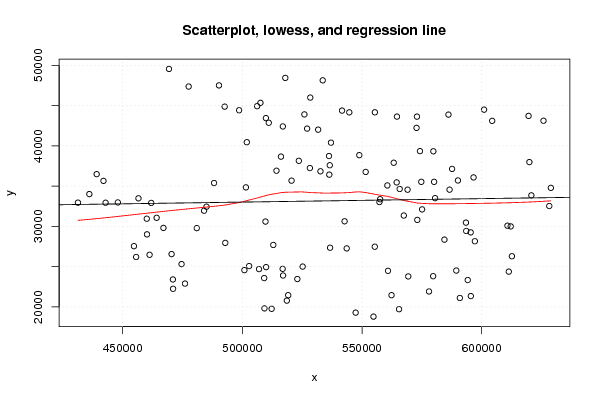
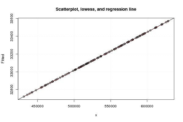
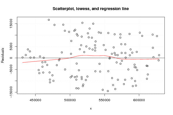
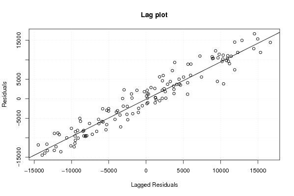
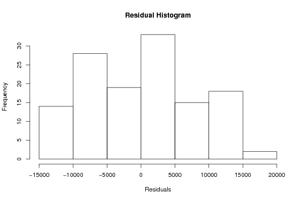
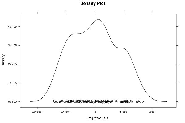
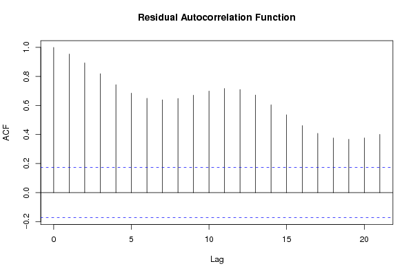
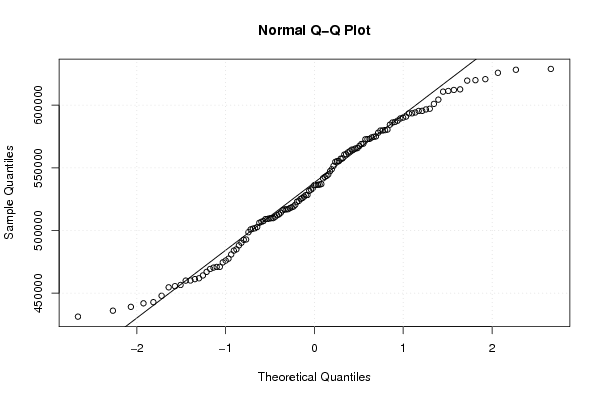
Figures (Output of Computation) | |||||||||||||||||||||||||||||||||||||||||||||||||||||||||||||
Input Parameters & R Code | |||||||||||||||||||||||||||||||||||||||||||||||||||||||||||||
| Parameters (Session): | |||||||||||||||||||||||||||||||||||||||||||||||||||||||||||||
| par1 = 0 ; | |||||||||||||||||||||||||||||||||||||||||||||||||||||||||||||
| Parameters (R input): | |||||||||||||||||||||||||||||||||||||||||||||||||||||||||||||
| par1 = 0 ; | |||||||||||||||||||||||||||||||||||||||||||||||||||||||||||||
| R code (references can be found in the software module): | |||||||||||||||||||||||||||||||||||||||||||||||||||||||||||||
par1 <- as.numeric(par1) | |||||||||||||||||||||||||||||||||||||||||||||||||||||||||||||