Free Statistics
of Irreproducible Research!
Description of Statistical Computation | |||||||||||||||||||||||||||||||||||||||||||||||||||||||||||||
|---|---|---|---|---|---|---|---|---|---|---|---|---|---|---|---|---|---|---|---|---|---|---|---|---|---|---|---|---|---|---|---|---|---|---|---|---|---|---|---|---|---|---|---|---|---|---|---|---|---|---|---|---|---|---|---|---|---|---|---|---|---|
| Author's title | |||||||||||||||||||||||||||||||||||||||||||||||||||||||||||||
| Author | *The author of this computation has been verified* | ||||||||||||||||||||||||||||||||||||||||||||||||||||||||||||
| R Software Module | rwasp_linear_regression.wasp | ||||||||||||||||||||||||||||||||||||||||||||||||||||||||||||
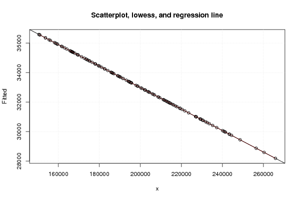
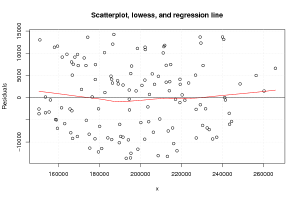
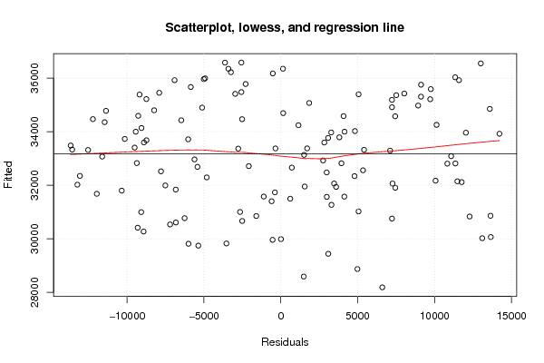
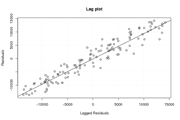
| Title produced by software | Linear Regression Graphical Model Validation | ||||||||||||||||||||||||||||||||||||||||||||||||||||||||||||
| Date of computation | Fri, 17 Dec 2010 13:47:08 +0000 | ||||||||||||||||||||||||||||||||||||||||||||||||||||||||||||
| Cite this page as follows | Statistical Computations at FreeStatistics.org, Office for Research Development and Education, URL https://freestatistics.org/blog/index.php?v=date/2010/Dec/17/t1292593522ujeh7kw9jl81t6m.htm/, Retrieved Tue, 13 Jan 2026 14:49:49 +0000 | ||||||||||||||||||||||||||||||||||||||||||||||||||||||||||||
| Statistical Computations at FreeStatistics.org, Office for Research Development and Education, URL https://freestatistics.org/blog/index.php?pk=111463, Retrieved Tue, 13 Jan 2026 14:49:49 +0000 | |||||||||||||||||||||||||||||||||||||||||||||||||||||||||||||
| QR Codes: | |||||||||||||||||||||||||||||||||||||||||||||||||||||||||||||
|
| |||||||||||||||||||||||||||||||||||||||||||||||||||||||||||||
| Original text written by user: | |||||||||||||||||||||||||||||||||||||||||||||||||||||||||||||
| IsPrivate? | No (this computation is public) | ||||||||||||||||||||||||||||||||||||||||||||||||||||||||||||
| User-defined keywords | |||||||||||||||||||||||||||||||||||||||||||||||||||||||||||||
| Estimated Impact | 469 | ||||||||||||||||||||||||||||||||||||||||||||||||||||||||||||
Tree of Dependent Computations | |||||||||||||||||||||||||||||||||||||||||||||||||||||||||||||
| Family? (F = Feedback message, R = changed R code, M = changed R Module, P = changed Parameters, D = changed Data) | |||||||||||||||||||||||||||||||||||||||||||||||||||||||||||||
| - [Linear Regression Graphical Model Validation] [Colombia Coffee -...] [2008-02-26 10:22:06] [74be16979710d4c4e7c6647856088456] - M D [Linear Regression Graphical Model Validation] [Scatterplot Tutorial] [2010-11-05 11:55:49] [aeb27d5c05332f2e597ad139ee63fbe4] - D [Linear Regression Graphical Model Validation] [Simple Linear Reg...] [2010-11-12 11:48:01] [aeb27d5c05332f2e597ad139ee63fbe4] - D [Linear Regression Graphical Model Validation] [Simple Linear Reg...] [2010-12-17 13:47:08] [18ef3d986e8801a4b28404e69e5bf56b] [Current] | |||||||||||||||||||||||||||||||||||||||||||||||||||||||||||||
| Feedback Forum | |||||||||||||||||||||||||||||||||||||||||||||||||||||||||||||
Post a new message | |||||||||||||||||||||||||||||||||||||||||||||||||||||||||||||
Dataset | |||||||||||||||||||||||||||||||||||||||||||||||||||||||||||||
| Dataseries X: | |||||||||||||||||||||||||||||||||||||||||||||||||||||||||||||
211868 229527 229139 198563 195722 202196 205816 212588 214320 220375 204442 206903 214126 226899 223532 195309 186005 188906 191563 189226 186413 178037 166827 169362 174330 187069 186530 158114 151001 159612 161914 164182 169701 171297 166444 173476 182516 202388 202300 168053 167302 172608 178106 185686 194581 194596 197922 208795 230580 240636 240048 211457 211142 214771 212610 219313 219277 231805 229245 241114 248624 265845 256446 219452 217142 221678 227184 230354 235243 237217 233575 244460 243324 260307 241476 203666 200237 204045 209465 213586 216234 213188 208679 217859 227247 243477 232571 191531 186029 189733 190420 194163 198770 195198 193111 195411 202108 215706 206348 166972 166070 169292 175041 177876 181140 179566 175335 184128 189917 194690 179612 150605 150569 153745 155511 159044 163095 159585 158644 166618 176512 200765 182698 153730 156145 161570 165688 173666 180144 | |||||||||||||||||||||||||||||||||||||||||||||||||||||||||||||
| Dataseries Y: | |||||||||||||||||||||||||||||||||||||||||||||||||||||||||||||
43880 43110 44496 44164 40399 36763 37903 35532 35533 32110 33374 35462 33508 36080 34560 38737 38144 37594 36424 36843 37246 38661 40454 44928 48441 48140 45998 47369 49554 47510 44873 45344 42413 36912 43452 42142 44382 43636 44167 44423 42868 43908 42013 38846 35087 33026 34646 37135 37985 43121 43722 43630 42234 39351 39327 35704 30466 28155 29257 29998 32529 34787 33855 34556 31348 30805 28353 24514 21106 21346 23335 24379 26290 30084 29429 30632 27349 27264 27474 24482 21453 18788 19282 19713 21917 23812 23785 24696 24562 23580 24939 23899 21454 19761 19815 20780 23462 25005 24725 26198 27543 26471 26558 25317 22896 22248 23406 25073 27691 30599 31948 32946 34012 32936 32974 30951 29812 29010 31068 32447 34844 35676 35387 36488 35652 33488 32914 29781 27951 | |||||||||||||||||||||||||||||||||||||||||||||||||||||||||||||
Tables (Output of Computation) | |||||||||||||||||||||||||||||||||||||||||||||||||||||||||||||
| |||||||||||||||||||||||||||||||||||||||||||||||||||||||||||||
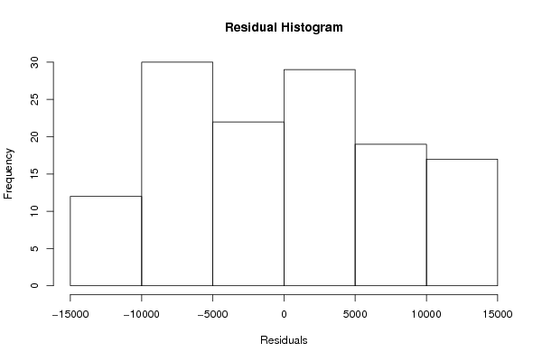
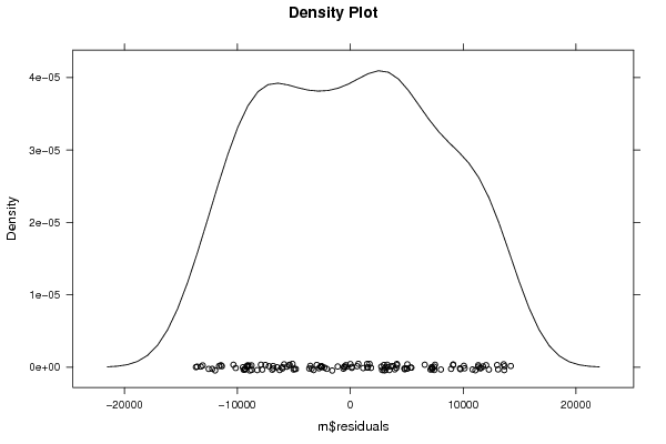
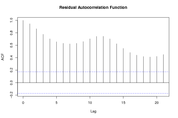
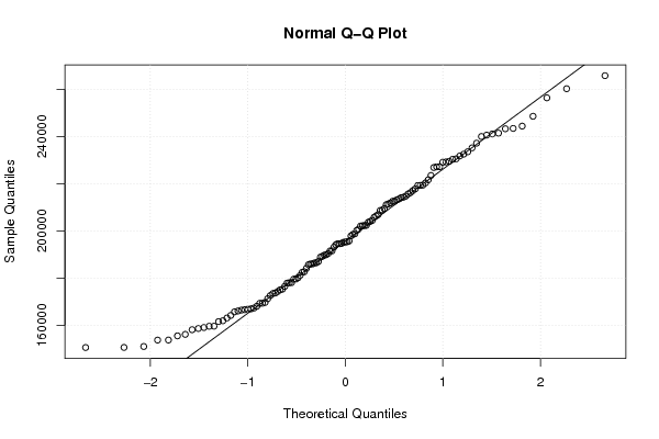
Figures (Output of Computation) | |||||||||||||||||||||||||||||||||||||||||||||||||||||||||||||
Input Parameters & R Code | |||||||||||||||||||||||||||||||||||||||||||||||||||||||||||||
| Parameters (Session): | |||||||||||||||||||||||||||||||||||||||||||||||||||||||||||||
| par1 = 0 ; | |||||||||||||||||||||||||||||||||||||||||||||||||||||||||||||
| Parameters (R input): | |||||||||||||||||||||||||||||||||||||||||||||||||||||||||||||
| par1 = 0 ; | |||||||||||||||||||||||||||||||||||||||||||||||||||||||||||||
| R code (references can be found in the software module): | |||||||||||||||||||||||||||||||||||||||||||||||||||||||||||||
par1 <- as.numeric(par1) | |||||||||||||||||||||||||||||||||||||||||||||||||||||||||||||