Free Statistics
of Irreproducible Research!
Description of Statistical Computation | |||||||||||||||||||||
|---|---|---|---|---|---|---|---|---|---|---|---|---|---|---|---|---|---|---|---|---|---|
| Author's title | |||||||||||||||||||||
| Author | *The author of this computation has been verified* | ||||||||||||||||||||
| R Software Module | rwasp_meanplot.wasp | ||||||||||||||||||||
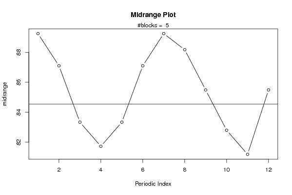
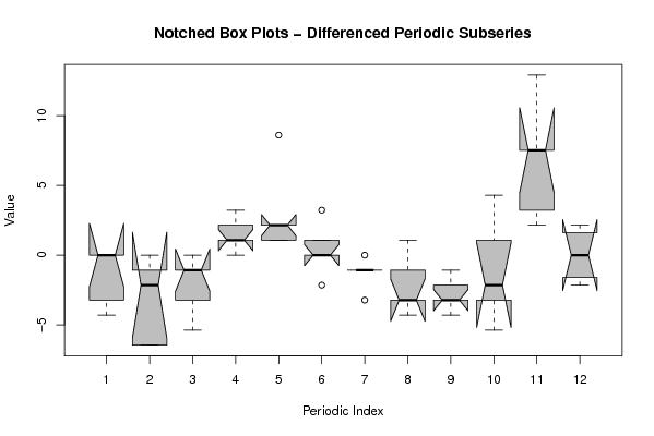
| Title produced by software | Mean Plot | ||||||||||||||||||||
| Date of computation | Sat, 07 Nov 2009 07:00:38 -0700 | ||||||||||||||||||||
| Cite this page as follows | Statistical Computations at FreeStatistics.org, Office for Research Development and Education, URL https://freestatistics.org/blog/index.php?v=date/2009/Nov/07/t1257602698uqzk20mq17e4njy.htm/, Retrieved Thu, 18 Sep 2025 08:27:34 +0000 | ||||||||||||||||||||
| Statistical Computations at FreeStatistics.org, Office for Research Development and Education, URL https://freestatistics.org/blog/index.php?pk=54410, Retrieved Thu, 18 Sep 2025 08:27:34 +0000 | |||||||||||||||||||||
| QR Codes: | |||||||||||||||||||||
|
| |||||||||||||||||||||
| Original text written by user: | |||||||||||||||||||||
| IsPrivate? | No (this computation is public) | ||||||||||||||||||||
| User-defined keywords | |||||||||||||||||||||
| Estimated Impact | 341 | ||||||||||||||||||||
Tree of Dependent Computations | |||||||||||||||||||||
| Family? (F = Feedback message, R = changed R code, M = changed R Module, P = changed Parameters, D = changed Data) | |||||||||||||||||||||
| - [Mean Plot] [3/11/2009] [2009-11-02 22:07:54] [b98453cac15ba1066b407e146608df68] - PD [Mean Plot] [ws 6] [2009-11-07 14:00:38] [f7d3e79b917995ba1c8c80042fc22ef9] [Current] | |||||||||||||||||||||
| Feedback Forum | |||||||||||||||||||||
Post a new message | |||||||||||||||||||||
Dataset | |||||||||||||||||||||
| Dataseries X: | |||||||||||||||||||||
100 100 93,5483871 88,17204301 89,24731183 91,39784946 92,47311828 91,39784946 88,17204301 87,09677419 84,94623656 92,47311828 93,5483871 93,5483871 91,39784946 90,32258065 91,39784946 93,5483871 93,5483871 92,47311828 91,39784946 89,24731183 86,02150538 88,17204301 87,09677419 87,09677419 86,02150538 84,94623656 84,94623656 86,02150538 86,02150538 84,94623656 86,02150538 82,79569892 77,41935484 80,64516129 78,49462366 75,2688172 75,2688172 75,2688172 77,41935484 78,49462366 76,34408602 73,11827957 68,8172043 65,59139785 69,89247312 82,79569892 84,94623656 80,64516129 74,19354839 70,96774194 74,19354839 82,79569892 86,02150538 86,02150538 82,79569892 78,49462366 79,56989247 87,09677419 | |||||||||||||||||||||
Tables (Output of Computation) | |||||||||||||||||||||
| |||||||||||||||||||||
Figures (Output of Computation) | |||||||||||||||||||||
Input Parameters & R Code | |||||||||||||||||||||
| Parameters (Session): | |||||||||||||||||||||
| par1 = 12 ; | |||||||||||||||||||||
| Parameters (R input): | |||||||||||||||||||||
| par1 = 12 ; | |||||||||||||||||||||
| R code (references can be found in the software module): | |||||||||||||||||||||
par1 <- as.numeric(par1) | |||||||||||||||||||||