Free Statistics
of Irreproducible Research!
Description of Statistical Computation | |||||||||||||||||||||
|---|---|---|---|---|---|---|---|---|---|---|---|---|---|---|---|---|---|---|---|---|---|
| Author's title | |||||||||||||||||||||
| Author | *The author of this computation has been verified* | ||||||||||||||||||||
| R Software Module | rwasp_meanplot.wasp | ||||||||||||||||||||
| Title produced by software | Mean Plot | ||||||||||||||||||||
| Date of computation | Mon, 02 Nov 2009 23:07:54 +0100 | ||||||||||||||||||||
| Cite this page as follows | Statistical Computations at FreeStatistics.org, Office for Research Development and Education, URL https://freestatistics.org/blog/index.php?v=date/2009/Nov/02/t12571997437cqg4ne9yvc8san.htm/, Retrieved Sat, 06 Jun 2026 08:09:45 +0000 | ||||||||||||||||||||
| Statistical Computations at FreeStatistics.org, Office for Research Development and Education, URL https://freestatistics.org/blog/index.php?pk=53038, Retrieved Sat, 06 Jun 2026 08:09:45 +0000 | |||||||||||||||||||||
| QR Codes: | |||||||||||||||||||||
|
| |||||||||||||||||||||
| Original text written by user: | |||||||||||||||||||||
| IsPrivate? | No (this computation is public) | ||||||||||||||||||||
| User-defined keywords | |||||||||||||||||||||
| Estimated Impact | 929 | ||||||||||||||||||||
Tree of Dependent Computations | |||||||||||||||||||||
| Family? (F = Feedback message, R = changed R code, M = changed R Module, P = changed Parameters, D = changed Data) | |||||||||||||||||||||
| - [Mean Plot] [3/11/2009] [2009-11-02 22:07:54] [d76b387543b13b5e3afd8ff9e5fdc89f] [Current] - PD [Mean Plot] [] [2009-11-04 15:42:39] [8d2349dc1d6314bc274adc9ad027c980] - PD [Mean Plot] [] [2009-11-04 15:47:29] [4d62210f0915d3a20cbf115865da7cd4] - R PD [Mean Plot] [ws6] [2009-11-04 15:55:03] [757146c69eaf0537be37c7b0c18216d8] - PD [Mean Plot] [mean plot] [2009-11-04 19:26:11] [315ba876df544ad397193b5931d5f354] - P [Mean Plot] [Paper] [2009-12-09 19:51:32] [3e19a07d230ba260a720e0e03e0f40f2] - D [Mean Plot] [ws 6 y] [2009-11-04 22:46:56] [6e4e01d7eb22a9f33d58ebb35753a195] - PD [Mean Plot] [mean plot] [2009-11-05 10:42:37] [cd6314e7e707a6546bd4604c9d1f2b69] - D [Mean Plot] [WS 6 Mean Plot - ...] [2009-11-05 10:49:18] [b103a1dc147def8132c7f643ad8c8f84] - D [Mean Plot] [Paper: Mean plot] [2009-12-17 12:33:22] [b103a1dc147def8132c7f643ad8c8f84] - PD [Mean Plot] [Mean Plot Y[t]] [2009-11-05 12:11:05] [4395c69e961f9a13a0559fd2f0a72538] - D [Mean Plot] [Paper Mean Plot Y[t]] [2009-12-17 16:30:24] [4395c69e961f9a13a0559fd2f0a72538] - PD [Mean Plot] [Mean Plot BDM] [2009-11-05 13:19:35] [f5d341d4bbba73282fc6e80153a6d315] - PD [Mean Plot] [Mean Plot BDM] [2009-11-10 12:01:58] [f5d341d4bbba73282fc6e80153a6d315] - [Mean Plot] [tg13] [2009-11-10 14:41:41] [a21bac9c8d3d56fdec8be4e719e2c7ed] - R P [Mean Plot] [ws6] [2009-11-15 22:38:36] [3fc64fd7a52ce121dfe13dba27bf6e5b] - [Mean Plot] [TVD 13] [2009-11-10 22:41:03] [42ad1186d39724f834063794eac7cea3] - [Mean Plot] [PA13] [2009-12-15 10:00:48] [a21bac9c8d3d56fdec8be4e719e2c7ed] - D [Mean Plot] [WS6 Mean plot] [2009-11-13 19:25:54] [445b292c553470d9fed8bc2796fd3a00] - RM D [Standard Deviation Plot] [WS6 Standard devi...] [2009-11-13 19:33:06] [445b292c553470d9fed8bc2796fd3a00] - PD [Mean Plot] [shwws6vr1] [2009-11-05 14:43:43] [2b2cfeea2f5ac2a1bcb842baaf1415ef] - PD [Mean Plot] [Shwws6v1] [2009-11-05 14:43:25] [5f89c040fdf1f8599c99d7f78a662321] - PD [Mean Plot] [mean plot] [2009-11-05 16:48:17] [eaf42bcf5162b5692bb3c7f9d4636222] - D [Mean Plot] [Shw6: Mean Plot v...] [2009-11-05 19:49:52] [3c8b83428ce260cd44df892bb7619588] - D [Mean Plot] [Shw6: Mean Plot v...] [2009-11-05 20:20:46] [3c8b83428ce260cd44df892bb7619588] - PD [Mean Plot] [] [2009-11-06 10:56:19] [74be16979710d4c4e7c6647856088456] - PD [Mean Plot] [ws6_mean plot] [2009-11-06 15:48:34] [8b1aef4e7013bd33fbc2a5833375c5f5] - [Mean Plot] [] [2009-11-11 10:32:54] [08fc5c07292c885b941f0cb515ce13f3] - D [Mean Plot] [Mean plot - uitvo...] [2009-12-10 22:29:43] [37a8d600db9abe09a2528d150ccff095] - RMPD [Standard Deviation-Mean Plot] [Standard deviatio...] [2009-12-10 23:53:58] [37a8d600db9abe09a2528d150ccff095] - D [Mean Plot] [Mean plot] [2009-11-07 09:31:45] [3b0db66ac8145b1be856a517e2900332] - PD [Mean Plot] [ws 6] [2009-11-07 14:00:38] [b5908418e3090fddbd22f5f0f774653d] - D [Mean Plot] [WS 6: Mean Plot] [2009-11-07 16:07:37] [8cf9233b7464ea02e32be3b30fdac052] - PD [Mean Plot] [WS 6: Mean plot] [2009-11-12 17:15:53] [b97b96148b0223bc16666763988dc147] - D [Mean Plot] [] [2009-11-07 16:10:51] [77305478ee09a4d442b7c3bff26eeaaa] - PD [Mean Plot] [SHWWS6link11] [2009-11-08 10:32:43] [a66d3a79ef9e5308cd94a469bc5ca464] - PD [Mean Plot] [Workshop 6 Mean Plot] [2009-11-08 12:17:28] [f924a0adda9c1905a1ba8f1c751261ff] - PD [Mean Plot] [Mean plot, Median...] [2009-11-08 14:19:47] [d46757a0a8c9b00540ab7e7e0c34bfc4] - RMPD [Standard Deviation Plot] [St. Deviation Plot] [2009-11-08 14:46:32] [d46757a0a8c9b00540ab7e7e0c34bfc4] - PD [Mean Plot] [] [2009-11-08 15:39:10] [7369a9baefff1ba9d2171738b4c9faa6] F PD [Mean Plot] [] [2009-11-08 16:21:01] [cf890101a20378422561610e0d41fd9c] - D [Mean Plot] [Mean plot] [2009-11-08 17:11:08] [e2a6b1b31bd881219e1879835b4c60d0] - PD [Mean Plot] [Mean Plot] [2009-12-13 20:09:01] [e2a6b1b31bd881219e1879835b4c60d0] - PD [Mean Plot] [WS 6 Mean Plot Y[t]] [2009-11-09 10:33:45] [83058a88a37d754675a5cd22dab372fc] - PD [Mean Plot] [Workshop 6] [2009-11-09 10:53:10] [3e19a07d230ba260a720e0e03e0f40f2] - D [Mean Plot] [WS6] [2009-11-15 14:12:34] [9f35ad889e41dd0c9322ca60d75b9f47] - PD [Mean Plot] [Mean Plot icp] [2009-11-09 12:26:45] [134dc66689e3d457a82860db6471d419] - PD [Mean Plot] [Mean Plot icp] [2009-11-09 12:26:45] [134dc66689e3d457a82860db6471d419] - RM [Standard Deviation Plot] [standard deviatio...] [2009-11-14 10:49:56] [ba905ddf7cdf9ecb063c35348c4dab2e] [Truncated] | |||||||||||||||||||||
| Feedback Forum | |||||||||||||||||||||
Post a new message | |||||||||||||||||||||
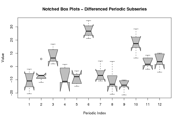
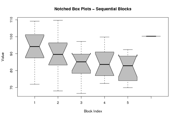
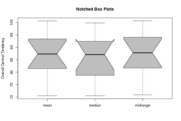
Dataset | |||||||||||||||||||||
| Dataseries X: | |||||||||||||||||||||
109.20 88.60 94.30 98.30 86.40 80.60 104.10 108.20 93.40 71.90 94.10 94.90 96.40 91.10 84.40 86.40 88.00 75.10 109.70 103.00 82.10 68.00 96.40 94.30 90.00 88.00 76.10 82.50 81.40 66.50 97.20 94.10 80.70 70.50 87.80 89.50 99.60 84.20 75.10 92.00 80.80 73.10 99.80 90.00 83.10 72.40 78.80 87.30 91.00 80.10 73.60 86.40 74.50 71.20 92.40 81.50 85.30 69.90 84.20 90.70 100.30 | |||||||||||||||||||||
Tables (Output of Computation) | |||||||||||||||||||||
| |||||||||||||||||||||
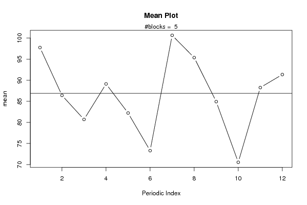
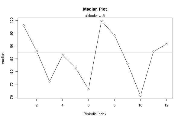
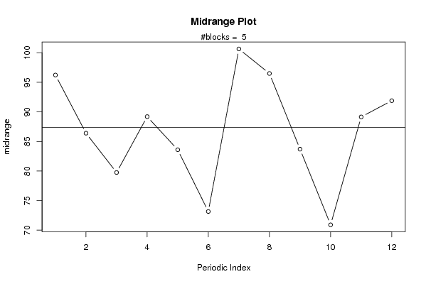
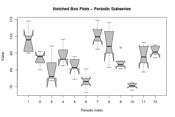
Figures (Output of Computation) | |||||||||||||||||||||
Input Parameters & R Code | |||||||||||||||||||||
| Parameters (Session): | |||||||||||||||||||||
| Parameters (R input): | |||||||||||||||||||||
| par1 = 12 ; | |||||||||||||||||||||
| R code (references can be found in the software module): | |||||||||||||||||||||
par1 <- as.numeric(par1) | |||||||||||||||||||||