Free Statistics
of Irreproducible Research!
Description of Statistical Computation | |||||||||||||||||||||||||||||||||||||||||||||||||||||||||||||||||
|---|---|---|---|---|---|---|---|---|---|---|---|---|---|---|---|---|---|---|---|---|---|---|---|---|---|---|---|---|---|---|---|---|---|---|---|---|---|---|---|---|---|---|---|---|---|---|---|---|---|---|---|---|---|---|---|---|---|---|---|---|---|---|---|---|---|
| Author's title | |||||||||||||||||||||||||||||||||||||||||||||||||||||||||||||||||
| Author | *The author of this computation has been verified* | ||||||||||||||||||||||||||||||||||||||||||||||||||||||||||||||||
| R Software Module | rwasp_edabi.wasp | ||||||||||||||||||||||||||||||||||||||||||||||||||||||||||||||||
| Title produced by software | Bivariate Explorative Data Analysis | ||||||||||||||||||||||||||||||||||||||||||||||||||||||||||||||||
| Date of computation | Wed, 04 Nov 2009 20:11:20 -0700 | ||||||||||||||||||||||||||||||||||||||||||||||||||||||||||||||||
| Cite this page as follows | Statistical Computations at FreeStatistics.org, Office for Research Development and Education, URL https://freestatistics.org/blog/index.php?v=date/2009/Nov/05/t1257390910mannuboyenx9xpd.htm/, Retrieved Thu, 03 Jul 2025 12:53:02 +0000 | ||||||||||||||||||||||||||||||||||||||||||||||||||||||||||||||||
| Statistical Computations at FreeStatistics.org, Office for Research Development and Education, URL https://freestatistics.org/blog/index.php?pk=53879, Retrieved Thu, 03 Jul 2025 12:53:02 +0000 | |||||||||||||||||||||||||||||||||||||||||||||||||||||||||||||||||
| QR Codes: | |||||||||||||||||||||||||||||||||||||||||||||||||||||||||||||||||
|
| |||||||||||||||||||||||||||||||||||||||||||||||||||||||||||||||||
| Original text written by user: | |||||||||||||||||||||||||||||||||||||||||||||||||||||||||||||||||
| IsPrivate? | No (this computation is public) | ||||||||||||||||||||||||||||||||||||||||||||||||||||||||||||||||
| User-defined keywords | WS 5 | ||||||||||||||||||||||||||||||||||||||||||||||||||||||||||||||||
| Estimated Impact | 284 | ||||||||||||||||||||||||||||||||||||||||||||||||||||||||||||||||
Tree of Dependent Computations | |||||||||||||||||||||||||||||||||||||||||||||||||||||||||||||||||
| Family? (F = Feedback message, R = changed R code, M = changed R Module, P = changed Parameters, D = changed Data) | |||||||||||||||||||||||||||||||||||||||||||||||||||||||||||||||||
| - [Univariate Data Series] [SHWWS2/1] [2009-10-12 16:52:29] [9717cb857c153ca3061376906953b329] - PD [Univariate Data Series] [Aantal niet-werke...] [2009-10-24 19:05:50] [9717cb857c153ca3061376906953b329] - MPD [Univariate Data Series] [Aantal inschrijvi...] [2009-11-05 03:01:41] [9717cb857c153ca3061376906953b329] - RMPD [Bivariate Explorative Data Analysis] [WS 5] [2009-11-05 03:11:20] [52b85b290d6f50b0921ad6729b8a5af2] [Current] - D [Bivariate Explorative Data Analysis] [WS 5] [2009-11-05 03:39:48] [9717cb857c153ca3061376906953b329] - RMPD [Trivariate Scatterplots] [WS 5] [2009-11-05 04:15:15] [9717cb857c153ca3061376906953b329] - RMP [Partial Correlation] [WS 5] [2009-11-05 04:24:39] [9717cb857c153ca3061376906953b329] - R D [Bivariate Explorative Data Analysis] [] [2011-11-22 17:33:37] [fbaf17a8836493f6de0f4e0e997711e1] - R D [Bivariate Explorative Data Analysis] [] [2011-11-22 17:44:12] [fbaf17a8836493f6de0f4e0e997711e1] | |||||||||||||||||||||||||||||||||||||||||||||||||||||||||||||||||
| Feedback Forum | |||||||||||||||||||||||||||||||||||||||||||||||||||||||||||||||||
Post a new message | |||||||||||||||||||||||||||||||||||||||||||||||||||||||||||||||||
Dataset | |||||||||||||||||||||||||||||||||||||||||||||||||||||||||||||||||
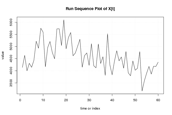
| Dataseries X: | |||||||||||||||||||||||||||||||||||||||||||||||||||||||||||||||||
4138 4634 3996 4308 4143 4429 5219 4929 5755 5592 4163 4962 5208 4755 4491 5732 5731 5040 6102 4904 5369 5578 4619 4731 5011 5299 4146 4625 4736 4219 5116 4205 4121 5103 4300 4578 3809 5526 4247 3830 4394 4826 4409 4569 4106 4794 3914 3793 4405 4022 4100 4788 3163 3585 3903 4178 3863 4187 4178 4354 | |||||||||||||||||||||||||||||||||||||||||||||||||||||||||||||||||
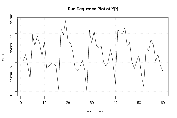
| Dataseries Y: | |||||||||||||||||||||||||||||||||||||||||||||||||||||||||||||||||
20366 22782 19169 13807 29743 25591 29096 26482 22405 27044 17970 18730 19684 19785 18479 10698 31956 29506 34506 27165 26736 23691 18157 17328 18205 20995 17382 9367 31124 26551 30651 25859 25100 25778 20418 18688 20424 24776 19814 12738 31566 30111 30019 31934 25826 26835 20205 17789 20520 22518 15572 11509 25447 24090 27786 26195 20516 22759 19028 16971 | |||||||||||||||||||||||||||||||||||||||||||||||||||||||||||||||||
Tables (Output of Computation) | |||||||||||||||||||||||||||||||||||||||||||||||||||||||||||||||||
| |||||||||||||||||||||||||||||||||||||||||||||||||||||||||||||||||
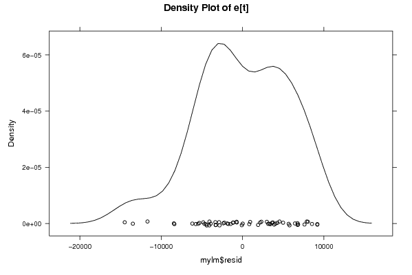
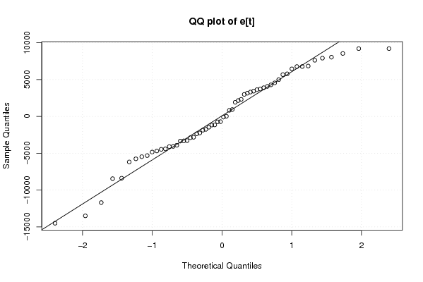
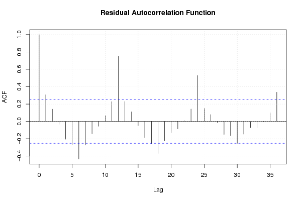
Figures (Output of Computation) | |||||||||||||||||||||||||||||||||||||||||||||||||||||||||||||||||
Input Parameters & R Code | |||||||||||||||||||||||||||||||||||||||||||||||||||||||||||||||||
| Parameters (Session): | |||||||||||||||||||||||||||||||||||||||||||||||||||||||||||||||||
| par1 = 0 ; par2 = 36 ; | |||||||||||||||||||||||||||||||||||||||||||||||||||||||||||||||||
| Parameters (R input): | |||||||||||||||||||||||||||||||||||||||||||||||||||||||||||||||||
| par1 = 0 ; par2 = 36 ; | |||||||||||||||||||||||||||||||||||||||||||||||||||||||||||||||||
| R code (references can be found in the software module): | |||||||||||||||||||||||||||||||||||||||||||||||||||||||||||||||||
par1 <- as.numeric(par1) | |||||||||||||||||||||||||||||||||||||||||||||||||||||||||||||||||