Free Statistics
of Irreproducible Research!
Description of Statistical Computation | |||||||||||||||||||||||||||||||||||||||||||||||||||||
|---|---|---|---|---|---|---|---|---|---|---|---|---|---|---|---|---|---|---|---|---|---|---|---|---|---|---|---|---|---|---|---|---|---|---|---|---|---|---|---|---|---|---|---|---|---|---|---|---|---|---|---|---|---|
| Author's title | |||||||||||||||||||||||||||||||||||||||||||||||||||||
| Author | *The author of this computation has been verified* | ||||||||||||||||||||||||||||||||||||||||||||||||||||
| R Software Module | rwasp_edauni.wasp | ||||||||||||||||||||||||||||||||||||||||||||||||||||
| Title produced by software | Univariate Explorative Data Analysis | ||||||||||||||||||||||||||||||||||||||||||||||||||||
| Date of computation | Wed, 04 Nov 2009 04:57:24 -0700 | ||||||||||||||||||||||||||||||||||||||||||||||||||||
| Cite this page as follows | Statistical Computations at FreeStatistics.org, Office for Research Development and Education, URL https://freestatistics.org/blog/index.php?v=date/2009/Nov/04/t1257335945u8q2mdqqvolka25.htm/, Retrieved Sun, 07 Dec 2025 05:17:58 +0000 | ||||||||||||||||||||||||||||||||||||||||||||||||||||
| Statistical Computations at FreeStatistics.org, Office for Research Development and Education, URL https://freestatistics.org/blog/index.php?pk=53575, Retrieved Sun, 07 Dec 2025 05:17:58 +0000 | |||||||||||||||||||||||||||||||||||||||||||||||||||||
| QR Codes: | |||||||||||||||||||||||||||||||||||||||||||||||||||||
|
| |||||||||||||||||||||||||||||||||||||||||||||||||||||
| Original text written by user: | |||||||||||||||||||||||||||||||||||||||||||||||||||||
| IsPrivate? | No (this computation is public) | ||||||||||||||||||||||||||||||||||||||||||||||||||||
| User-defined keywords | |||||||||||||||||||||||||||||||||||||||||||||||||||||
| Estimated Impact | 424 | ||||||||||||||||||||||||||||||||||||||||||||||||||||
Tree of Dependent Computations | |||||||||||||||||||||||||||||||||||||||||||||||||||||
| Family? (F = Feedback message, R = changed R code, M = changed R Module, P = changed Parameters, D = changed Data) | |||||||||||||||||||||||||||||||||||||||||||||||||||||
| - [Notched Boxplots] [3/11/2009] [2009-11-02 21:10:41] [b98453cac15ba1066b407e146608df68] - D [Notched Boxplots] [ws 6 1] [2009-11-04 11:54:28] [6e4e01d7eb22a9f33d58ebb35753a195] - RMPD [Univariate Explorative Data Analysis] [ws 6 kla] [2009-11-04 11:57:24] [2e4ef2c1b76db9b31c0a03b96e94ad77] [Current] - [Univariate Explorative Data Analysis] [ws 6 sto] [2009-11-04 11:59:43] [6e4e01d7eb22a9f33d58ebb35753a195] - D [Univariate Explorative Data Analysis] [ws 6 sch] [2009-11-04 12:01:28] [6e4e01d7eb22a9f33d58ebb35753a195] - D [Univariate Explorative Data Analysis] [ws 6 totpr] [2009-11-04 12:02:45] [6e4e01d7eb22a9f33d58ebb35753a195] - RMPD [Notched Boxplots] [WS6_notched_boxplots] [2009-11-09 14:00:59] [2c75a4273e8c314249ceca659377406c] - RMPD [Kendall tau Correlation Matrix] [WS6_kendall_tau] [2009-11-09 14:05:52] [2c75a4273e8c314249ceca659377406c] - RMPD [Partial Correlation] [WS6_partial_corre...] [2009-11-09 14:12:10] [2c75a4273e8c314249ceca659377406c] - RMPD [Box-Cox Linearity Plot] [WS6_boxcox] [2009-11-09 14:16:08] [2c75a4273e8c314249ceca659377406c] | |||||||||||||||||||||||||||||||||||||||||||||||||||||
| Feedback Forum | |||||||||||||||||||||||||||||||||||||||||||||||||||||
Post a new message | |||||||||||||||||||||||||||||||||||||||||||||||||||||
Dataset | |||||||||||||||||||||||||||||||||||||||||||||||||||||
| Dataseries X: | |||||||||||||||||||||||||||||||||||||||||||||||||||||
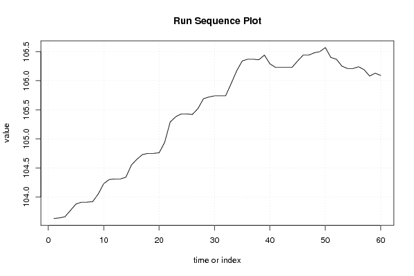
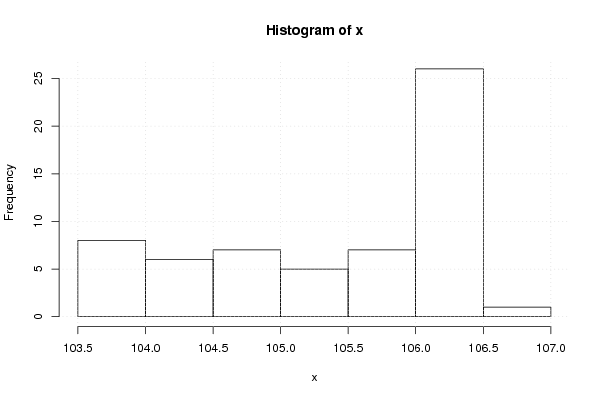
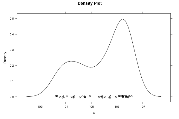
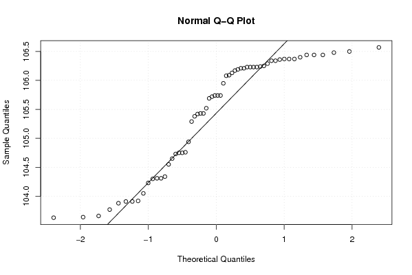
103.63 103.64 103.66 103.77 103.88 103.91 103.91 103.92 104.05 104.23 104.30 104.31 104.31 104.34 104.55 104.65 104.73 104.75 104.75 104.76 104.94 105.29 105.38 105.43 105.43 105.42 105.52 105.69 105.72 105.74 105.74 105.74 105.95 106.17 106.34 106.37 106.37 106.36 106.44 106.29 106.23 106.23 106.23 106.23 106.34 106.44 106.44 106.48 106.50 106.57 106.40 106.37 106.25 106.21 106.21 106.24 106.19 106.08 106.13 106.09 | |||||||||||||||||||||||||||||||||||||||||||||||||||||
Tables (Output of Computation) | |||||||||||||||||||||||||||||||||||||||||||||||||||||
| |||||||||||||||||||||||||||||||||||||||||||||||||||||
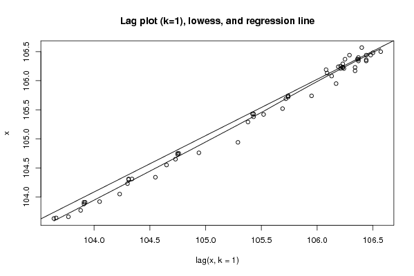
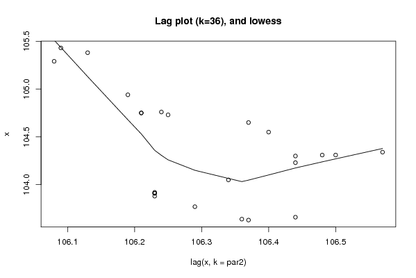
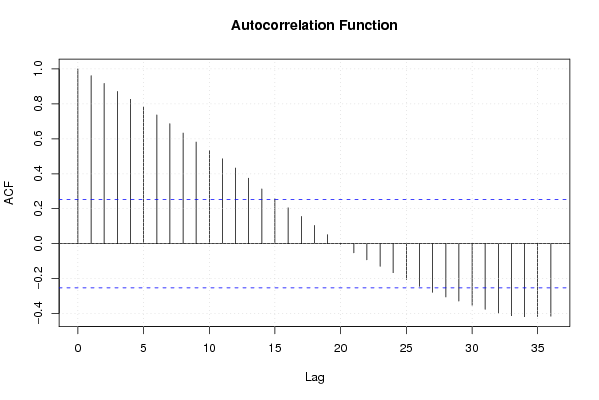
Figures (Output of Computation) | |||||||||||||||||||||||||||||||||||||||||||||||||||||
Input Parameters & R Code | |||||||||||||||||||||||||||||||||||||||||||||||||||||
| Parameters (Session): | |||||||||||||||||||||||||||||||||||||||||||||||||||||
| par1 = 0 ; par2 = 36 ; | |||||||||||||||||||||||||||||||||||||||||||||||||||||
| Parameters (R input): | |||||||||||||||||||||||||||||||||||||||||||||||||||||
| par1 = 0 ; par2 = 36 ; | |||||||||||||||||||||||||||||||||||||||||||||||||||||
| R code (references can be found in the software module): | |||||||||||||||||||||||||||||||||||||||||||||||||||||
par1 <- as.numeric(par1) | |||||||||||||||||||||||||||||||||||||||||||||||||||||