Free Statistics
of Irreproducible Research!
Description of Statistical Computation | |||||||||||||||||||||||||||||||||||||||||||||||||||||||||||||||||||||||||||||||||||||||||||||||||||||||||||||||||||||||||||||||||||||||||||||
|---|---|---|---|---|---|---|---|---|---|---|---|---|---|---|---|---|---|---|---|---|---|---|---|---|---|---|---|---|---|---|---|---|---|---|---|---|---|---|---|---|---|---|---|---|---|---|---|---|---|---|---|---|---|---|---|---|---|---|---|---|---|---|---|---|---|---|---|---|---|---|---|---|---|---|---|---|---|---|---|---|---|---|---|---|---|---|---|---|---|---|---|---|---|---|---|---|---|---|---|---|---|---|---|---|---|---|---|---|---|---|---|---|---|---|---|---|---|---|---|---|---|---|---|---|---|---|---|---|---|---|---|---|---|---|---|---|---|---|---|---|---|
| Author's title | |||||||||||||||||||||||||||||||||||||||||||||||||||||||||||||||||||||||||||||||||||||||||||||||||||||||||||||||||||||||||||||||||||||||||||||
| Author | *The author of this computation has been verified* | ||||||||||||||||||||||||||||||||||||||||||||||||||||||||||||||||||||||||||||||||||||||||||||||||||||||||||||||||||||||||||||||||||||||||||||
| R Software Module | rwasp_notchedbox1.wasp | ||||||||||||||||||||||||||||||||||||||||||||||||||||||||||||||||||||||||||||||||||||||||||||||||||||||||||||||||||||||||||||||||||||||||||||
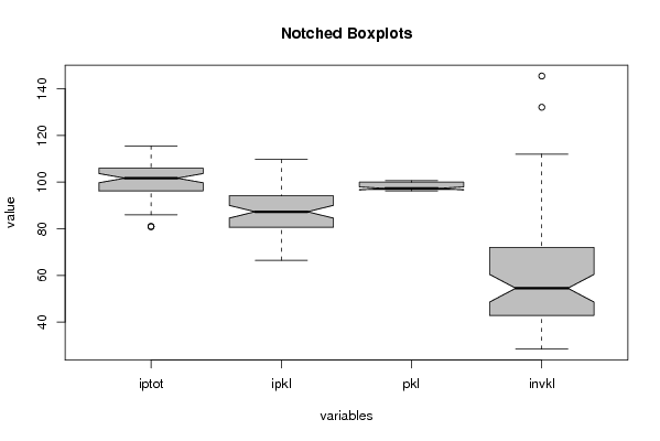
| Title produced by software | Notched Boxplots | ||||||||||||||||||||||||||||||||||||||||||||||||||||||||||||||||||||||||||||||||||||||||||||||||||||||||||||||||||||||||||||||||||||||||||||
| Date of computation | Mon, 02 Nov 2009 22:10:41 +0100 | ||||||||||||||||||||||||||||||||||||||||||||||||||||||||||||||||||||||||||||||||||||||||||||||||||||||||||||||||||||||||||||||||||||||||||||
| Cite this page as follows | Statistical Computations at FreeStatistics.org, Office for Research Development and Education, URL https://freestatistics.org/blog/index.php?v=date/2009/Nov/02/t1257196349n7pyjc3lkf9f67n.htm/, Retrieved Sat, 30 May 2026 03:02:43 +0000 | ||||||||||||||||||||||||||||||||||||||||||||||||||||||||||||||||||||||||||||||||||||||||||||||||||||||||||||||||||||||||||||||||||||||||||||
| Statistical Computations at FreeStatistics.org, Office for Research Development and Education, URL https://freestatistics.org/blog/index.php?pk=52983, Retrieved Sat, 30 May 2026 03:02:43 +0000 | |||||||||||||||||||||||||||||||||||||||||||||||||||||||||||||||||||||||||||||||||||||||||||||||||||||||||||||||||||||||||||||||||||||||||||||
| QR Codes: | |||||||||||||||||||||||||||||||||||||||||||||||||||||||||||||||||||||||||||||||||||||||||||||||||||||||||||||||||||||||||||||||||||||||||||||
|
| |||||||||||||||||||||||||||||||||||||||||||||||||||||||||||||||||||||||||||||||||||||||||||||||||||||||||||||||||||||||||||||||||||||||||||||
| Original text written by user: | |||||||||||||||||||||||||||||||||||||||||||||||||||||||||||||||||||||||||||||||||||||||||||||||||||||||||||||||||||||||||||||||||||||||||||||
| IsPrivate? | No (this computation is public) | ||||||||||||||||||||||||||||||||||||||||||||||||||||||||||||||||||||||||||||||||||||||||||||||||||||||||||||||||||||||||||||||||||||||||||||
| User-defined keywords | |||||||||||||||||||||||||||||||||||||||||||||||||||||||||||||||||||||||||||||||||||||||||||||||||||||||||||||||||||||||||||||||||||||||||||||
| Estimated Impact | 1162 | ||||||||||||||||||||||||||||||||||||||||||||||||||||||||||||||||||||||||||||||||||||||||||||||||||||||||||||||||||||||||||||||||||||||||||||
Tree of Dependent Computations | |||||||||||||||||||||||||||||||||||||||||||||||||||||||||||||||||||||||||||||||||||||||||||||||||||||||||||||||||||||||||||||||||||||||||||||
| Family? (F = Feedback message, R = changed R code, M = changed R Module, P = changed Parameters, D = changed Data) | |||||||||||||||||||||||||||||||||||||||||||||||||||||||||||||||||||||||||||||||||||||||||||||||||||||||||||||||||||||||||||||||||||||||||||||
| - [Notched Boxplots] [3/11/2009] [2009-11-02 21:10:41] [d76b387543b13b5e3afd8ff9e5fdc89f] [Current] - RMPD [Univariate Explorative Data Analysis] [tijdreeks 1] [2009-11-03 12:01:52] [214e6e00abbde49700521a7ef1d30da2] - RMPD [Univariate Explorative Data Analysis] [tijdreeks 2] [2009-11-03 12:03:53] [214e6e00abbde49700521a7ef1d30da2] - RMPD [Univariate Explorative Data Analysis] [tijdreeks 3] [2009-11-03 12:05:38] [214e6e00abbde49700521a7ef1d30da2] - RMPD [Univariate Explorative Data Analysis] [Tijdreeks 4] [2009-11-03 12:07:52] [214e6e00abbde49700521a7ef1d30da2] - D [Univariate Explorative Data Analysis] [Multivariate Tijd...] [2009-12-05 14:27:17] [214e6e00abbde49700521a7ef1d30da2] - D [Univariate Explorative Data Analysis] [Multivariate Tijd...] [2009-12-05 14:29:00] [214e6e00abbde49700521a7ef1d30da2] - D [Univariate Explorative Data Analysis] [Multivariate Tijd...] [2009-12-05 14:30:27] [214e6e00abbde49700521a7ef1d30da2] - D [Univariate Explorative Data Analysis] [Multivariate Tijd...] [2009-12-05 14:31:47] [214e6e00abbde49700521a7ef1d30da2] - RMPD [Back to Back Histogram] [Back To Back Hist...] [2009-12-05 14:36:09] [214e6e00abbde49700521a7ef1d30da2] - RMPD [Kendall tau Correlation Matrix] [Kendal Tau Correl...] [2009-12-05 14:42:32] [214e6e00abbde49700521a7ef1d30da2] - RM D [Box-Cox Linearity Plot] [Box Cox Lineairit...] [2009-12-06 15:47:52] [214e6e00abbde49700521a7ef1d30da2] - RMPD [Bivariate Kernel Density Estimation] [Bivariate Kernal ...] [2009-12-10 16:40:47] [214e6e00abbde49700521a7ef1d30da2] - RMPD [Back to Back Histogram] [BacktoBack] [2009-11-03 12:12:21] [214e6e00abbde49700521a7ef1d30da2] - RMPD [Kendall tau Correlation Matrix] [Kendall Tau Corre...] [2009-11-03 14:17:34] [214e6e00abbde49700521a7ef1d30da2] - RM D [Box-Cox Linearity Plot] [Box cox linairity...] [2009-11-03 14:36:05] [214e6e00abbde49700521a7ef1d30da2] - RMP [Bagplot] [Bagplot] [2009-11-03 18:19:37] [214e6e00abbde49700521a7ef1d30da2] - D [Bagplot] [Bag plot] [2009-11-05 09:51:07] [214e6e00abbde49700521a7ef1d30da2] - D [Bagplot] [Bagplot] [2009-11-05 18:46:57] [214e6e00abbde49700521a7ef1d30da2] - RMP [Bivariate Kernel Density Estimation] [Bivariate kernal ...] [2009-11-03 18:21:13] [214e6e00abbde49700521a7ef1d30da2] - D [Bivariate Kernel Density Estimation] [Bivariate kernal ...] [2009-11-05 09:43:54] [214e6e00abbde49700521a7ef1d30da2] - RM [Kendall tau Rank Correlation] [Kendall Rank corr...] [2009-11-03 18:23:38] [214e6e00abbde49700521a7ef1d30da2] - RMP [Bivariate Explorative Data Analysis] [Bivariate EDA] [2009-11-03 18:31:55] [214e6e00abbde49700521a7ef1d30da2] - D [Box-Cox Linearity Plot] [Box Cox lineairit...] [2009-11-05 09:38:08] [214e6e00abbde49700521a7ef1d30da2] - RM D [Box-Cox Linearity Plot] [Box coc linairity...] [2009-11-03 14:39:06] [214e6e00abbde49700521a7ef1d30da2] - D [Notched Boxplots] [] [2009-11-03 20:37:41] [74be16979710d4c4e7c6647856088456] - D [Notched Boxplots] [Workshop 5.3] [2009-11-03 21:27:11] [d31db4f83c6a129f6d3e47077769e868] - D [Notched Boxplots] [Workshop 5.4] [2009-11-03 21:34:49] [d31db4f83c6a129f6d3e47077769e868] - D [Notched Boxplots] [Workshop 5 Notche...] [2009-11-04 10:59:20] [f924a0adda9c1905a1ba8f1c751261ff] - D [Notched Boxplots] [ws 6 1] [2009-11-04 11:54:28] [6e4e01d7eb22a9f33d58ebb35753a195] - RMPD [Univariate Explorative Data Analysis] [ws 6 kla] [2009-11-04 11:57:24] [6e4e01d7eb22a9f33d58ebb35753a195] - [Univariate Explorative Data Analysis] [ws 6 sto] [2009-11-04 11:59:43] [6e4e01d7eb22a9f33d58ebb35753a195] - D [Univariate Explorative Data Analysis] [ws 6 sch] [2009-11-04 12:01:28] [6e4e01d7eb22a9f33d58ebb35753a195] - D [Univariate Explorative Data Analysis] [ws 6 totpr] [2009-11-04 12:02:45] [6e4e01d7eb22a9f33d58ebb35753a195] - RMPD [Notched Boxplots] [WS6_notched_boxplots] [2009-11-09 14:00:59] [2c75a4273e8c314249ceca659377406c] - RMPD [Kendall tau Correlation Matrix] [WS6_kendall_tau] [2009-11-09 14:05:52] [2c75a4273e8c314249ceca659377406c] - RMPD [Partial Correlation] [WS6_partial_corre...] [2009-11-09 14:12:10] [2c75a4273e8c314249ceca659377406c] - RMPD [Box-Cox Linearity Plot] [WS6_boxcox] [2009-11-09 14:16:08] [2c75a4273e8c314249ceca659377406c] - D [Notched Boxplots] [] [2009-11-04 14:57:15] [8d2349dc1d6314bc274adc9ad027c980] F D [Notched Boxplots] [] [2009-11-04 14:58:21] [4d62210f0915d3a20cbf115865da7cd4] - D [Notched Boxplots] [notched boxplot] [2009-11-16 18:32:43] [ed603017d2bee8fbd82b6d5ec04e12c3] - D [Notched Boxplots] [WS 6 Review] [2009-11-20 12:01:20] [830e13ac5e5ac1e5b21c6af0c149b21d] - R D [Notched Boxplots] [Notched boxplots ...] [2009-11-04 15:00:59] [757146c69eaf0537be37c7b0c18216d8] - D [Notched Boxplots] [notched boxplot] [2009-11-04 16:42:15] [315ba876df544ad397193b5931d5f354] - RMPD [Trivariate Scatterplots] [WS5 Trivariate sc...] [2009-11-04 16:43:18] [445b292c553470d9fed8bc2796fd3a00] F RMPD [Partial Correlation] [WS5 Partial corre...] [2009-11-04 16:54:40] [445b292c553470d9fed8bc2796fd3a00] - RMPD [Trivariate Scatterplots] [WS5 Trivariate sc...] [2009-11-04 16:57:18] [445b292c553470d9fed8bc2796fd3a00] - D [Notched Boxplots] [box plot notched] [2009-11-04 17:44:31] [315ba876df544ad397193b5931d5f354] - [Notched Boxplots] [Paper] [2009-12-07 10:14:57] [3e19a07d230ba260a720e0e03e0f40f2] [Truncated] | |||||||||||||||||||||||||||||||||||||||||||||||||||||||||||||||||||||||||||||||||||||||||||||||||||||||||||||||||||||||||||||||||||||||||||||
| Feedback Forum | |||||||||||||||||||||||||||||||||||||||||||||||||||||||||||||||||||||||||||||||||||||||||||||||||||||||||||||||||||||||||||||||||||||||||||||
Post a new message | |||||||||||||||||||||||||||||||||||||||||||||||||||||||||||||||||||||||||||||||||||||||||||||||||||||||||||||||||||||||||||||||||||||||||||||
Dataset | |||||||||||||||||||||||||||||||||||||||||||||||||||||||||||||||||||||||||||||||||||||||||||||||||||||||||||||||||||||||||||||||||||||||||||||
| Dataseries X: | |||||||||||||||||||||||||||||||||||||||||||||||||||||||||||||||||||||||||||||||||||||||||||||||||||||||||||||||||||||||||||||||||||||||||||||
110.40 109.20 99.90 72.50 96.40 88.60 99.80 59.40 101.90 94.30 99.80 85.70 106.20 98.30 100.30 88.20 81.00 86.40 99.90 62.80 94.70 80.60 99.90 87.00 101.00 104.10 100.00 79.20 109.40 108.20 100.10 112.00 102.30 93.40 100.10 79.20 90.70 71.90 100.20 132.10 96.20 94.10 100.30 40.10 96.10 94.90 100.60 69.00 106.00 96.40 100.00 59.40 103.10 91.10 100.10 73.80 102.00 84.40 100.20 57.40 104.70 86.40 100.00 81.10 86.00 88.00 100.10 46.60 92.10 75.10 100.10 41.40 106.90 109.70 100.10 71.20 112.60 103.00 100.50 67.90 101.70 82.10 100.50 72.00 92.00 68.00 100.50 145.50 97.40 96.40 96.30 39.70 97.00 94.30 96.30 51.90 105.40 90.00 96.80 73.70 102.70 88.00 96.80 70.90 98.10 76.10 96.90 60.80 104.50 82.50 96.80 61.00 87.40 81.40 96.80 54.50 89.90 66.50 96.80 39.10 109.80 97.20 96.80 66.60 111.70 94.10 97.00 58.50 98.60 80.70 97.00 59.80 96.90 70.50 97.00 80.90 95.10 87.80 96.80 37.30 97.00 89.50 96.90 44.60 112.70 99.60 97.20 48.70 102.90 84.20 97.30 54.00 97.40 75.10 97.30 49.50 111.40 92.00 97.20 61.60 87.40 80.80 97.30 35.00 96.80 73.10 97.30 35.70 114.10 99.80 97.30 51.30 110.30 90.00 97.30 49.00 103.90 83.10 97.30 41.50 101.60 72.40 97.30 72.50 94.60 78.80 98.10 42.10 95.90 87.30 96.80 44.10 104.70 91.00 96.80 45.10 102.80 80.10 96.80 50.30 98.10 73.60 96.80 40.90 113.90 86.40 96.80 47.20 80.90 74.50 96.80 36.90 95.70 71.20 96.80 40.90 113.20 92.40 96.80 38.30 105.90 81.50 96.80 46.30 108.80 85.30 96.80 28.40 102.30 69.90 96.80 78.40 99.00 84.20 96.90 36.80 100.70 90.70 97.10 50.70 115.50 100.30 97.10 42.80 | |||||||||||||||||||||||||||||||||||||||||||||||||||||||||||||||||||||||||||||||||||||||||||||||||||||||||||||||||||||||||||||||||||||||||||||
Tables (Output of Computation) | |||||||||||||||||||||||||||||||||||||||||||||||||||||||||||||||||||||||||||||||||||||||||||||||||||||||||||||||||||||||||||||||||||||||||||||
| |||||||||||||||||||||||||||||||||||||||||||||||||||||||||||||||||||||||||||||||||||||||||||||||||||||||||||||||||||||||||||||||||||||||||||||
Figures (Output of Computation) | |||||||||||||||||||||||||||||||||||||||||||||||||||||||||||||||||||||||||||||||||||||||||||||||||||||||||||||||||||||||||||||||||||||||||||||
Input Parameters & R Code | |||||||||||||||||||||||||||||||||||||||||||||||||||||||||||||||||||||||||||||||||||||||||||||||||||||||||||||||||||||||||||||||||||||||||||||
| Parameters (Session): | |||||||||||||||||||||||||||||||||||||||||||||||||||||||||||||||||||||||||||||||||||||||||||||||||||||||||||||||||||||||||||||||||||||||||||||
| par1 = grey ; | |||||||||||||||||||||||||||||||||||||||||||||||||||||||||||||||||||||||||||||||||||||||||||||||||||||||||||||||||||||||||||||||||||||||||||||
| Parameters (R input): | |||||||||||||||||||||||||||||||||||||||||||||||||||||||||||||||||||||||||||||||||||||||||||||||||||||||||||||||||||||||||||||||||||||||||||||
| par1 = grey ; | |||||||||||||||||||||||||||||||||||||||||||||||||||||||||||||||||||||||||||||||||||||||||||||||||||||||||||||||||||||||||||||||||||||||||||||
| R code (references can be found in the software module): | |||||||||||||||||||||||||||||||||||||||||||||||||||||||||||||||||||||||||||||||||||||||||||||||||||||||||||||||||||||||||||||||||||||||||||||
z <- as.data.frame(t(y)) | |||||||||||||||||||||||||||||||||||||||||||||||||||||||||||||||||||||||||||||||||||||||||||||||||||||||||||||||||||||||||||||||||||||||||||||