Free Statistics
of Irreproducible Research!
Description of Statistical Computation | |||||||||||||||||||||
|---|---|---|---|---|---|---|---|---|---|---|---|---|---|---|---|---|---|---|---|---|---|
| Author's title | |||||||||||||||||||||
| Author | *The author of this computation has been verified* | ||||||||||||||||||||
| R Software Module | rwasp_meanplot.wasp | ||||||||||||||||||||
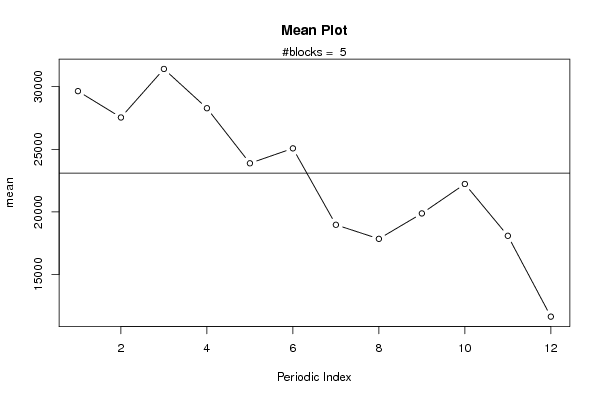
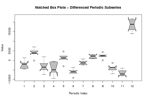
| Title produced by software | Mean Plot | ||||||||||||||||||||
| Date of computation | Wed, 30 Dec 2009 07:08:44 -0700 | ||||||||||||||||||||
| Cite this page as follows | Statistical Computations at FreeStatistics.org, Office for Research Development and Education, URL https://freestatistics.org/blog/index.php?v=date/2009/Dec/30/t1262182160wn35u20b675sszl.htm/, Retrieved Tue, 01 Jul 2025 11:16:18 +0000 | ||||||||||||||||||||
| Statistical Computations at FreeStatistics.org, Office for Research Development and Education, URL https://freestatistics.org/blog/index.php?pk=71288, Retrieved Tue, 01 Jul 2025 11:16:18 +0000 | |||||||||||||||||||||
| QR Codes: | |||||||||||||||||||||
|
| |||||||||||||||||||||
| Original text written by user: | |||||||||||||||||||||
| IsPrivate? | No (this computation is public) | ||||||||||||||||||||
| User-defined keywords | |||||||||||||||||||||
| Estimated Impact | 257 | ||||||||||||||||||||
Tree of Dependent Computations | |||||||||||||||||||||
| Family? (F = Feedback message, R = changed R code, M = changed R Module, P = changed Parameters, D = changed Data) | |||||||||||||||||||||
| - [Bivariate Data Series] [Bivariate dataset] [2008-01-05 23:51:08] [74be16979710d4c4e7c6647856088456] F RMPD [Mean Plot] [Colombia Coffee] [2008-01-07 13:38:24] [74be16979710d4c4e7c6647856088456] - PD [Mean Plot] [Notched boxplot -...] [2008-12-07 09:49:05] [c45c87b96bbf32ffc2144fc37d767b2e] - D [Mean Plot] [Notched boxplot -...] [2008-12-14 12:56:52] [74be16979710d4c4e7c6647856088456] - D [Mean Plot] [Notched boxplot -...] [2008-12-16 21:22:54] [c45c87b96bbf32ffc2144fc37d767b2e] - M D [Mean Plot] [] [2009-12-30 10:19:42] [d2d412c7f4d35ffbf5ee5ee89db327d4] - D [Mean Plot] [] [2009-12-30 14:08:44] [f6a332ba2d530c028d935c5a5bbb53af] [Current] | |||||||||||||||||||||
| Feedback Forum | |||||||||||||||||||||
Post a new message | |||||||||||||||||||||
Dataset | |||||||||||||||||||||
| Dataseries X: | |||||||||||||||||||||
28029 29383 36438 32034 22679 24319 18004 17537 20366 22782 19169 13807 29743 25591 29096 26482 22405 27044 17970 18730 19684 19785 18479 10698 31956 29506 34506 27165 26736 23691 18157 17328 18205 20995 17382 9367 31124 26551 30651 25859 25100 25778 20418 18688 20424 24776 19814 12738 31566 30111 30019 31934 25826 26835 20205 17789 20520 22518 15572 11509 25447 24090 27786 26195 20516 22759 19028 16971 20036 22485 | |||||||||||||||||||||
Tables (Output of Computation) | |||||||||||||||||||||
| |||||||||||||||||||||
Figures (Output of Computation) | |||||||||||||||||||||
Input Parameters & R Code | |||||||||||||||||||||
| Parameters (Session): | |||||||||||||||||||||
| par1 = 12 ; | |||||||||||||||||||||
| Parameters (R input): | |||||||||||||||||||||
| par1 = 12 ; | |||||||||||||||||||||
| R code (references can be found in the software module): | |||||||||||||||||||||
par1 <- as.numeric(par1) | |||||||||||||||||||||