Free Statistics
of Irreproducible Research!
Description of Statistical Computation | |||||||||||||||||||||
|---|---|---|---|---|---|---|---|---|---|---|---|---|---|---|---|---|---|---|---|---|---|
| Author's title | |||||||||||||||||||||
| Author | *Unverified author* | ||||||||||||||||||||
| R Software Module | rwasp_meanplot.wasp | ||||||||||||||||||||
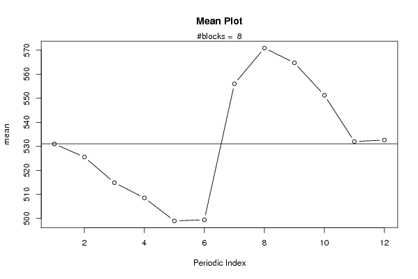
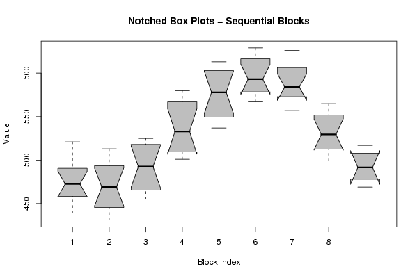
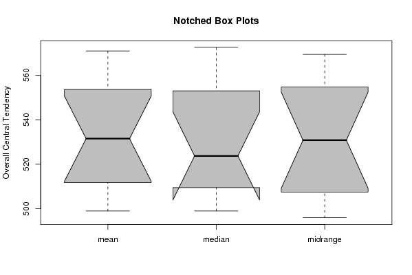
| Title produced by software | Mean Plot | ||||||||||||||||||||
| Date of computation | Sun, 14 Dec 2008 05:56:52 -0700 | ||||||||||||||||||||
| Cite this page as follows | Statistical Computations at FreeStatistics.org, Office for Research Development and Education, URL https://freestatistics.org/blog/index.php?v=date/2008/Dec/14/t1229260121c8h5aqwl2b2xce3.htm/, Retrieved Tue, 16 Sep 2025 13:34:49 +0000 | ||||||||||||||||||||
| Statistical Computations at FreeStatistics.org, Office for Research Development and Education, URL https://freestatistics.org/blog/index.php?pk=33346, Retrieved Tue, 16 Sep 2025 13:34:49 +0000 | |||||||||||||||||||||
| QR Codes: | |||||||||||||||||||||
|
| |||||||||||||||||||||
| Original text written by user: | |||||||||||||||||||||
| IsPrivate? | No (this computation is public) | ||||||||||||||||||||
| User-defined keywords | |||||||||||||||||||||
| Estimated Impact | 371 | ||||||||||||||||||||
Tree of Dependent Computations | |||||||||||||||||||||
| Family? (F = Feedback message, R = changed R code, M = changed R Module, P = changed Parameters, D = changed Data) | |||||||||||||||||||||
| - [Bivariate Data Series] [Bivariate dataset] [2008-01-05 23:51:08] [74be16979710d4c4e7c6647856088456] F RMPD [Mean Plot] [Colombia Coffee] [2008-01-07 13:38:24] [74be16979710d4c4e7c6647856088456] - PD [Mean Plot] [Notched boxplot -...] [2008-12-07 09:49:05] [c45c87b96bbf32ffc2144fc37d767b2e] - D [Mean Plot] [Notched boxplot -...] [2008-12-14 12:56:52] [d41d8cd98f00b204e9800998ecf8427e] [Current] - D [Mean Plot] [Notched boxplot -...] [2008-12-16 21:22:54] [c45c87b96bbf32ffc2144fc37d767b2e] - M D [Mean Plot] [] [2009-12-30 10:19:42] [d2d412c7f4d35ffbf5ee5ee89db327d4] - D [Mean Plot] [] [2009-12-30 14:08:44] [d2d412c7f4d35ffbf5ee5ee89db327d4] | |||||||||||||||||||||
| Feedback Forum | |||||||||||||||||||||
Post a new message | |||||||||||||||||||||
Dataset | |||||||||||||||||||||
| Dataseries X: | |||||||||||||||||||||
493 481 462 457 442 439 488 521 501 485 464 460 467 460 448 443 436 431 484 510 513 503 471 471 476 475 470 461 455 456 517 525 523 519 509 512 519 517 510 509 501 507 569 580 578 565 547 555 562 561 555 544 537 543 594 611 613 611 594 595 591 589 584 573 567 569 621 629 628 612 595 597 593 590 580 574 573 573 620 626 620 588 566 557 561 549 532 526 511 499 555 565 542 527 510 514 517 508 493 490 469 478 | |||||||||||||||||||||
Tables (Output of Computation) | |||||||||||||||||||||
| |||||||||||||||||||||
Figures (Output of Computation) | |||||||||||||||||||||
Input Parameters & R Code | |||||||||||||||||||||
| Parameters (Session): | |||||||||||||||||||||
| par1 = 12 ; | |||||||||||||||||||||
| Parameters (R input): | |||||||||||||||||||||
| par1 = 12 ; | |||||||||||||||||||||
| R code (references can be found in the software module): | |||||||||||||||||||||
par1 <- as.numeric(par1) | |||||||||||||||||||||