Repository of Reproducible Computations

Free Statistics

of Irreproducible Research!

Author's title

Author

*Unverified author*

R Software Module

rwasp_autocorrelation.wasp

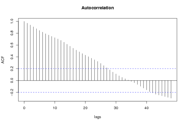
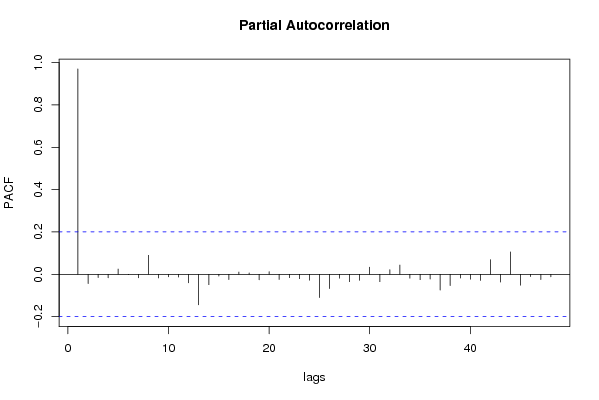
Title produced by software

(Partial) Autocorrelation Function

Date of computation

Thu, 11 Dec 2008 01:24:21 -0700

Cite this page as follows

Statistical Computations at FreeStatistics.org, Office for Research Development and Education, URL https://freestatistics.org/blog/index.php?v=date/2008/Dec/11/t1228983906wqdzqwa2bizxrje.htm/, Retrieved Wed, 15 May 2024 13:38:57 +0000

Statistical Computations at FreeStatistics.org, Office for Research Development and Education, URL https://freestatistics.org/blog/index.php?pk=32149, Retrieved Wed, 15 May 2024 13:38:57 +0000

QR Codes:

Paste this QR Code to cite your computation.

Original text written by user:

IsPrivate?

No (this computation is public)

User-defined keywords

Estimated Impact

246

Family? (F = Feedback message, R = changed R code, M = changed R Module, P = changed Parameters, D = changed Data)

-     [Harrell-Davis Quantiles] [Harrel davis deci...] [2008-10-18 16:19:32] [ea79f99c5895b39ae8bb6e8c563d0f54]
-   PD  [Harrell-Davis Quantiles] [Harrel davis deci...] [2008-10-18 17:17:36] [ea79f99c5895b39ae8bb6e8c563d0f54]
- RMPD      [(Partial) Autocorrelation Function] [OEF 2 deel 1 De L...] [2008-12-11 08:24:21] [1eda150a0abaa7374d7583f55f7b1e6e] [Current]
-   P         [(Partial) Autocorrelation Function] [0ef2 6bis AUTOCOR...] [2008-12-11 22:20:06] [74be16979710d4c4e7c6647856088456] 
-   P         [(Partial) Autocorrelation Function] [oef 2 opg6 autocorr] [2008-12-11 22:22:27] [74be16979710d4c4e7c6647856088456] 
- RMP         [Bootstrap Plot - Central Tendency] [Oef 2 opg. 7 De L...] [2008-12-18 22:45:41] [ea79f99c5895b39ae8bb6e8c563d0f54] 
- RMP           [Blocked Bootstrap Plot - Central Tendency] [VERbetering Block...] [2009-01-04 16:07:05] [ea79f99c5895b39ae8bb6e8c563d0f54] 
- RMP             [Variability] [SDL OPG 8 OEF3 va...] [2009-01-06 10:22:38] [ea79f99c5895b39ae8bb6e8c563d0f54] 
- RMP               [Classical Decomposition] [SDL OPG 9 OEF2] [2009-01-15 22:26:39] [74be16979710d4c4e7c6647856088456] 
- RMP                 [Exponential Smoothing] [SDL OPG 10 OEF2] [2009-01-17 11:19:26] [74be16979710d4c4e7c6647856088456] 
- RMP             [Standard Deviation Plot] [SDL OPG 8 OEF3 st...] [2009-01-06 10:27:14] [ea79f99c5895b39ae8bb6e8c563d0f54] 
- RMP             [Standard Deviation-Mean Plot] [SDL OPG 8 OEF3 st...] [2009-01-06 10:33:01] [ea79f99c5895b39ae8bb6e8c563d0f54] 
- RMP           [Blocked Bootstrap Plot - Central Tendency] [VERbetering Block...] [2009-01-04 16:22:41] [ea79f99c5895b39ae8bb6e8c563d0f54] 
- RMP           [Blocked Bootstrap Plot - Central Tendency] [VERbetering Block...] [2009-01-04 16:26:26] [ea79f99c5895b39ae8bb6e8c563d0f54] 
- RMP         [Bootstrap Plot - Central Tendency] [Oef 2 opg. 7 De L...] [2008-12-18 22:48:05] [ea79f99c5895b39ae8bb6e8c563d0f54] 
- RMP         [Bootstrap Plot - Central Tendency] [Oef 2 opg. 7 De L...] [2008-12-18 22:49:55] [ea79f99c5895b39ae8bb6e8c563d0f54] 

Feedback Forum

Post a new message

Dataseries X:

Download CSV

Histogram

Boxplots

Summary of computational transaction
Raw Input	view raw input (R code)
Raw Output	view raw output of R engine
Computing time	1 seconds
R Server	'Gwilym Jenkins' @ 72.249.127.135

\begin{tabular}{lllllllll}
\hline
Summary of computational transaction \tabularnewline
Raw Input & view raw input (R code)  \tabularnewline
Raw Output & view raw output of R engine  \tabularnewline
Computing time & 1 seconds \tabularnewline
R Server & 'Gwilym Jenkins' @ 72.249.127.135 \tabularnewline
\hline
\end{tabular}
%Source: https://freestatistics.org/blog/index.php?pk=32149&T=0

[TABLE]
[ROW][C]Summary of computational transaction[/C][/ROW]
[ROW][C]Raw Input[/C][C]view raw input (R code) [/C][/ROW]
[ROW][C]Raw Output[/C][C]view raw output of R engine [/C][/ROW]
[ROW][C]Computing time[/C][C]1 seconds[/C][/ROW]
[ROW][C]R Server[/C][C]'Gwilym Jenkins' @ 72.249.127.135[/C][/ROW]
[/TABLE]
Source: https://freestatistics.org/blog/index.php?pk=32149&T=0

Globally Unique Identifier (entire table): ba.freestatistics.org/blog/index.php?pk=32149&T=0

As an alternative you can also use a QR Code:

The GUIDs for individual cells are displayed in the table below:

Summary of computational transaction
Raw Input	view raw input (R code)
Raw Output	view raw output of R engine
Computing time	1 seconds
R Server	'Gwilym Jenkins' @ 72.249.127.135

Autocorrelation Function
Time lag k	ACF(k)	T-STAT	P-value
1	0.970235	9.5063	0
2	0.938798	9.1983	0
3	0.907362	8.8903	0
4	0.875926	8.5823	0
5	0.846916	8.298	0
6	0.81884	8.023	0
7	0.790764	7.7479	0
8	0.768853	7.5332	0
9	0.746941	7.3185	0
10	0.72503	7.1038	0
11	0.703119	6.8891	0
12	0.679165	6.6544	0
13	0.647428	6.3435	0
14	0.613626	6.0123	0
15	0.579824	5.6811	0
16	0.546023	5.3499	0
17	0.514648	5.0425	1e-06
18	0.48514	4.7534	4e-06
19	0.455632	4.4643	1.1e-05
20	0.429494	4.2082	2.9e-05
21	0.403356	3.9521	7.4e-05
22	0.377218	3.696	0.000182
23	0.35108	3.4399	0.000431
24	0.323526	3.1699	0.001023
25	0.289556	2.8371	0.002777
26	0.252676	2.4757	0.007525
27	0.215795	2.1144	0.018538
28	0.178915	1.753	0.041397
29	0.143155	1.4026	0.081977
30	0.111689	1.0943	0.138276
31	0.080222	0.786	0.216897
32	0.053256	0.5218	0.301506
33	0.030769	0.3015	0.381852
34	0.008282	0.0811	0.467746
35	-0.014204	-0.1392	0.444802
36	-0.03753	-0.3677	0.356946
37	-0.066147	-0.6481	0.259231
38	-0.096804	-0.9485	0.172633
39	-0.127461	-1.2489	0.107378
40	-0.158117	-1.5492	0.062309
41	-0.187467	-1.8368	0.034667
42	-0.209909	-2.0567	0.021215
43	-0.232352	-2.2766	0.012516
44	-0.245458	-2.405	0.009045
45	-0.258564	-2.5334	0.006458
46	-0.27167	-2.6618	0.004556
47	-0.284775	-2.7902	0.003177
48	-0.298223	-2.922	0.002168

\begin{tabular}{lllllllll}
\hline
Autocorrelation Function \tabularnewline
Time lag k & ACF(k) & T-STAT & P-value \tabularnewline
1 & 0.970235 & 9.5063 & 0 \tabularnewline
2 & 0.938798 & 9.1983 & 0 \tabularnewline
3 & 0.907362 & 8.8903 & 0 \tabularnewline
4 & 0.875926 & 8.5823 & 0 \tabularnewline
5 & 0.846916 & 8.298 & 0 \tabularnewline
6 & 0.81884 & 8.023 & 0 \tabularnewline
7 & 0.790764 & 7.7479 & 0 \tabularnewline
8 & 0.768853 & 7.5332 & 0 \tabularnewline
9 & 0.746941 & 7.3185 & 0 \tabularnewline
10 & 0.72503 & 7.1038 & 0 \tabularnewline
11 & 0.703119 & 6.8891 & 0 \tabularnewline
12 & 0.679165 & 6.6544 & 0 \tabularnewline
13 & 0.647428 & 6.3435 & 0 \tabularnewline
14 & 0.613626 & 6.0123 & 0 \tabularnewline
15 & 0.579824 & 5.6811 & 0 \tabularnewline
16 & 0.546023 & 5.3499 & 0 \tabularnewline
17 & 0.514648 & 5.0425 & 1e-06 \tabularnewline
18 & 0.48514 & 4.7534 & 4e-06 \tabularnewline
19 & 0.455632 & 4.4643 & 1.1e-05 \tabularnewline
20 & 0.429494 & 4.2082 & 2.9e-05 \tabularnewline
21 & 0.403356 & 3.9521 & 7.4e-05 \tabularnewline
22 & 0.377218 & 3.696 & 0.000182 \tabularnewline
23 & 0.35108 & 3.4399 & 0.000431 \tabularnewline
24 & 0.323526 & 3.1699 & 0.001023 \tabularnewline
25 & 0.289556 & 2.8371 & 0.002777 \tabularnewline
26 & 0.252676 & 2.4757 & 0.007525 \tabularnewline
27 & 0.215795 & 2.1144 & 0.018538 \tabularnewline
28 & 0.178915 & 1.753 & 0.041397 \tabularnewline
29 & 0.143155 & 1.4026 & 0.081977 \tabularnewline
30 & 0.111689 & 1.0943 & 0.138276 \tabularnewline
31 & 0.080222 & 0.786 & 0.216897 \tabularnewline
32 & 0.053256 & 0.5218 & 0.301506 \tabularnewline
33 & 0.030769 & 0.3015 & 0.381852 \tabularnewline
34 & 0.008282 & 0.0811 & 0.467746 \tabularnewline
35 & -0.014204 & -0.1392 & 0.444802 \tabularnewline
36 & -0.03753 & -0.3677 & 0.356946 \tabularnewline
37 & -0.066147 & -0.6481 & 0.259231 \tabularnewline
38 & -0.096804 & -0.9485 & 0.172633 \tabularnewline
39 & -0.127461 & -1.2489 & 0.107378 \tabularnewline
40 & -0.158117 & -1.5492 & 0.062309 \tabularnewline
41 & -0.187467 & -1.8368 & 0.034667 \tabularnewline
42 & -0.209909 & -2.0567 & 0.021215 \tabularnewline
43 & -0.232352 & -2.2766 & 0.012516 \tabularnewline
44 & -0.245458 & -2.405 & 0.009045 \tabularnewline
45 & -0.258564 & -2.5334 & 0.006458 \tabularnewline
46 & -0.27167 & -2.6618 & 0.004556 \tabularnewline
47 & -0.284775 & -2.7902 & 0.003177 \tabularnewline
48 & -0.298223 & -2.922 & 0.002168 \tabularnewline
\hline
\end{tabular}
%Source: https://freestatistics.org/blog/index.php?pk=32149&T=1

[TABLE]
[ROW][C]Autocorrelation Function[/C][/ROW]
[ROW][C]Time lag k[/C][C]ACF(k)[/C][C]T-STAT[/C][C]P-value[/C][/ROW]
[ROW][C]1[/C][C]0.970235[/C][C]9.5063[/C][C]0[/C][/ROW]
[ROW][C]2[/C][C]0.938798[/C][C]9.1983[/C][C]0[/C][/ROW]
[ROW][C]3[/C][C]0.907362[/C][C]8.8903[/C][C]0[/C][/ROW]
[ROW][C]4[/C][C]0.875926[/C][C]8.5823[/C][C]0[/C][/ROW]
[ROW][C]5[/C][C]0.846916[/C][C]8.298[/C][C]0[/C][/ROW]
[ROW][C]6[/C][C]0.81884[/C][C]8.023[/C][C]0[/C][/ROW]
[ROW][C]7[/C][C]0.790764[/C][C]7.7479[/C][C]0[/C][/ROW]
[ROW][C]8[/C][C]0.768853[/C][C]7.5332[/C][C]0[/C][/ROW]
[ROW][C]9[/C][C]0.746941[/C][C]7.3185[/C][C]0[/C][/ROW]
[ROW][C]10[/C][C]0.72503[/C][C]7.1038[/C][C]0[/C][/ROW]
[ROW][C]11[/C][C]0.703119[/C][C]6.8891[/C][C]0[/C][/ROW]
[ROW][C]12[/C][C]0.679165[/C][C]6.6544[/C][C]0[/C][/ROW]
[ROW][C]13[/C][C]0.647428[/C][C]6.3435[/C][C]0[/C][/ROW]
[ROW][C]14[/C][C]0.613626[/C][C]6.0123[/C][C]0[/C][/ROW]
[ROW][C]15[/C][C]0.579824[/C][C]5.6811[/C][C]0[/C][/ROW]
[ROW][C]16[/C][C]0.546023[/C][C]5.3499[/C][C]0[/C][/ROW]
[ROW][C]17[/C][C]0.514648[/C][C]5.0425[/C][C]1e-06[/C][/ROW]
[ROW][C]18[/C][C]0.48514[/C][C]4.7534[/C][C]4e-06[/C][/ROW]
[ROW][C]19[/C][C]0.455632[/C][C]4.4643[/C][C]1.1e-05[/C][/ROW]
[ROW][C]20[/C][C]0.429494[/C][C]4.2082[/C][C]2.9e-05[/C][/ROW]
[ROW][C]21[/C][C]0.403356[/C][C]3.9521[/C][C]7.4e-05[/C][/ROW]
[ROW][C]22[/C][C]0.377218[/C][C]3.696[/C][C]0.000182[/C][/ROW]
[ROW][C]23[/C][C]0.35108[/C][C]3.4399[/C][C]0.000431[/C][/ROW]
[ROW][C]24[/C][C]0.323526[/C][C]3.1699[/C][C]0.001023[/C][/ROW]
[ROW][C]25[/C][C]0.289556[/C][C]2.8371[/C][C]0.002777[/C][/ROW]
[ROW][C]26[/C][C]0.252676[/C][C]2.4757[/C][C]0.007525[/C][/ROW]
[ROW][C]27[/C][C]0.215795[/C][C]2.1144[/C][C]0.018538[/C][/ROW]
[ROW][C]28[/C][C]0.178915[/C][C]1.753[/C][C]0.041397[/C][/ROW]
[ROW][C]29[/C][C]0.143155[/C][C]1.4026[/C][C]0.081977[/C][/ROW]
[ROW][C]30[/C][C]0.111689[/C][C]1.0943[/C][C]0.138276[/C][/ROW]
[ROW][C]31[/C][C]0.080222[/C][C]0.786[/C][C]0.216897[/C][/ROW]
[ROW][C]32[/C][C]0.053256[/C][C]0.5218[/C][C]0.301506[/C][/ROW]
[ROW][C]33[/C][C]0.030769[/C][C]0.3015[/C][C]0.381852[/C][/ROW]
[ROW][C]34[/C][C]0.008282[/C][C]0.0811[/C][C]0.467746[/C][/ROW]
[ROW][C]35[/C][C]-0.014204[/C][C]-0.1392[/C][C]0.444802[/C][/ROW]
[ROW][C]36[/C][C]-0.03753[/C][C]-0.3677[/C][C]0.356946[/C][/ROW]
[ROW][C]37[/C][C]-0.066147[/C][C]-0.6481[/C][C]0.259231[/C][/ROW]
[ROW][C]38[/C][C]-0.096804[/C][C]-0.9485[/C][C]0.172633[/C][/ROW]
[ROW][C]39[/C][C]-0.127461[/C][C]-1.2489[/C][C]0.107378[/C][/ROW]
[ROW][C]40[/C][C]-0.158117[/C][C]-1.5492[/C][C]0.062309[/C][/ROW]
[ROW][C]41[/C][C]-0.187467[/C][C]-1.8368[/C][C]0.034667[/C][/ROW]
[ROW][C]42[/C][C]-0.209909[/C][C]-2.0567[/C][C]0.021215[/C][/ROW]
[ROW][C]43[/C][C]-0.232352[/C][C]-2.2766[/C][C]0.012516[/C][/ROW]
[ROW][C]44[/C][C]-0.245458[/C][C]-2.405[/C][C]0.009045[/C][/ROW]
[ROW][C]45[/C][C]-0.258564[/C][C]-2.5334[/C][C]0.006458[/C][/ROW]
[ROW][C]46[/C][C]-0.27167[/C][C]-2.6618[/C][C]0.004556[/C][/ROW]
[ROW][C]47[/C][C]-0.284775[/C][C]-2.7902[/C][C]0.003177[/C][/ROW]
[ROW][C]48[/C][C]-0.298223[/C][C]-2.922[/C][C]0.002168[/C][/ROW]
[/TABLE]
Source: https://freestatistics.org/blog/index.php?pk=32149&T=1

Globally Unique Identifier (entire table): ba.freestatistics.org/blog/index.php?pk=32149&T=1

As an alternative you can also use a QR Code:

The GUIDs for individual cells are displayed in the table below:

Autocorrelation Function
Time lag k	ACF(k)	T-STAT	P-value
1	0.970235	9.5063	0
2	0.938798	9.1983	0
3	0.907362	8.8903	0
4	0.875926	8.5823	0
5	0.846916	8.298	0
6	0.81884	8.023	0
7	0.790764	7.7479	0
8	0.768853	7.5332	0
9	0.746941	7.3185	0
10	0.72503	7.1038	0
11	0.703119	6.8891	0
12	0.679165	6.6544	0
13	0.647428	6.3435	0
14	0.613626	6.0123	0
15	0.579824	5.6811	0
16	0.546023	5.3499	0
17	0.514648	5.0425	1e-06
18	0.48514	4.7534	4e-06
19	0.455632	4.4643	1.1e-05
20	0.429494	4.2082	2.9e-05
21	0.403356	3.9521	7.4e-05
22	0.377218	3.696	0.000182
23	0.35108	3.4399	0.000431
24	0.323526	3.1699	0.001023
25	0.289556	2.8371	0.002777
26	0.252676	2.4757	0.007525
27	0.215795	2.1144	0.018538
28	0.178915	1.753	0.041397
29	0.143155	1.4026	0.081977
30	0.111689	1.0943	0.138276
31	0.080222	0.786	0.216897
32	0.053256	0.5218	0.301506
33	0.030769	0.3015	0.381852
34	0.008282	0.0811	0.467746
35	-0.014204	-0.1392	0.444802
36	-0.03753	-0.3677	0.356946
37	-0.066147	-0.6481	0.259231
38	-0.096804	-0.9485	0.172633
39	-0.127461	-1.2489	0.107378
40	-0.158117	-1.5492	0.062309
41	-0.187467	-1.8368	0.034667
42	-0.209909	-2.0567	0.021215
43	-0.232352	-2.2766	0.012516
44	-0.245458	-2.405	0.009045
45	-0.258564	-2.5334	0.006458
46	-0.27167	-2.6618	0.004556
47	-0.284775	-2.7902	0.003177
48	-0.298223	-2.922	0.002168

Partial Autocorrelation Function
Time lag k	PACF(k)	T-STAT	P-value
1	0.970235	9.5063	0
2	-0.043606	-0.4272	0.335078
3	-0.015438	-0.1513	0.440043
4	-0.016504	-0.1617	0.435939
5	0.024727	0.2423	0.404544
6	-0.002054	-0.0201	0.491993
7	-0.016298	-0.1597	0.436732
8	0.089677	0.8787	0.190891
9	-0.017171	-0.1682	0.433374
10	-0.011693	-0.1146	0.454513
11	-0.013055	-0.1279	0.449244
12	-0.040256	-0.3944	0.34707
13	-0.144359	-1.4144	0.080236
14	-0.048954	-0.4796	0.316285
15	-0.008489	-0.0832	0.466942
16	-0.024718	-0.2422	0.404575
17	0.010629	0.1041	0.458637
18	0.006598	0.0646	0.474295
19	-0.026154	-0.2563	0.39915
20	0.012382	0.1213	0.451848
21	-0.024254	-0.2376	0.406332
22	-0.016031	-0.1571	0.43776
23	-0.020575	-0.2016	0.420329
24	-0.027599	-0.2704	0.39371
25	-0.109876	-1.0766	0.142187
26	-0.067441	-0.6608	0.255166
27	-0.018572	-0.182	0.427997
28	-0.034724	-0.3402	0.367214
29	-0.028083	-0.2752	0.391893
30	0.033719	0.3304	0.370917
31	-0.035085	-0.3438	0.365889
32	0.021654	0.2122	0.416215
33	0.04401	0.4312	0.333642
34	-0.018208	-0.1784	0.429392
35	-0.025606	-0.2509	0.401219
36	-0.022555	-0.221	0.412784
37	-0.074555	-0.7305	0.233436
38	-0.053443	-0.5236	0.30087
39	-0.017734	-0.1738	0.43121
40	-0.022846	-0.2238	0.411678
41	-0.028748	-0.2817	0.389399
42	0.069193	0.6779	0.249718
43	-0.036818	-0.3607	0.359543
44	0.105982	1.0384	0.150845
45	-0.051667	-0.5062	0.306927
46	-0.0104	-0.1019	0.459526
47	-0.024694	-0.242	0.404666
48	-0.011557	-0.1132	0.455041

\begin{tabular}{lllllllll}
\hline
Partial Autocorrelation Function \tabularnewline
Time lag k & PACF(k) & T-STAT & P-value \tabularnewline
1 & 0.970235 & 9.5063 & 0 \tabularnewline
2 & -0.043606 & -0.4272 & 0.335078 \tabularnewline
3 & -0.015438 & -0.1513 & 0.440043 \tabularnewline
4 & -0.016504 & -0.1617 & 0.435939 \tabularnewline
5 & 0.024727 & 0.2423 & 0.404544 \tabularnewline
6 & -0.002054 & -0.0201 & 0.491993 \tabularnewline
7 & -0.016298 & -0.1597 & 0.436732 \tabularnewline
8 & 0.089677 & 0.8787 & 0.190891 \tabularnewline
9 & -0.017171 & -0.1682 & 0.433374 \tabularnewline
10 & -0.011693 & -0.1146 & 0.454513 \tabularnewline
11 & -0.013055 & -0.1279 & 0.449244 \tabularnewline
12 & -0.040256 & -0.3944 & 0.34707 \tabularnewline
13 & -0.144359 & -1.4144 & 0.080236 \tabularnewline
14 & -0.048954 & -0.4796 & 0.316285 \tabularnewline
15 & -0.008489 & -0.0832 & 0.466942 \tabularnewline
16 & -0.024718 & -0.2422 & 0.404575 \tabularnewline
17 & 0.010629 & 0.1041 & 0.458637 \tabularnewline
18 & 0.006598 & 0.0646 & 0.474295 \tabularnewline
19 & -0.026154 & -0.2563 & 0.39915 \tabularnewline
20 & 0.012382 & 0.1213 & 0.451848 \tabularnewline
21 & -0.024254 & -0.2376 & 0.406332 \tabularnewline
22 & -0.016031 & -0.1571 & 0.43776 \tabularnewline
23 & -0.020575 & -0.2016 & 0.420329 \tabularnewline
24 & -0.027599 & -0.2704 & 0.39371 \tabularnewline
25 & -0.109876 & -1.0766 & 0.142187 \tabularnewline
26 & -0.067441 & -0.6608 & 0.255166 \tabularnewline
27 & -0.018572 & -0.182 & 0.427997 \tabularnewline
28 & -0.034724 & -0.3402 & 0.367214 \tabularnewline
29 & -0.028083 & -0.2752 & 0.391893 \tabularnewline
30 & 0.033719 & 0.3304 & 0.370917 \tabularnewline
31 & -0.035085 & -0.3438 & 0.365889 \tabularnewline
32 & 0.021654 & 0.2122 & 0.416215 \tabularnewline
33 & 0.04401 & 0.4312 & 0.333642 \tabularnewline
34 & -0.018208 & -0.1784 & 0.429392 \tabularnewline
35 & -0.025606 & -0.2509 & 0.401219 \tabularnewline
36 & -0.022555 & -0.221 & 0.412784 \tabularnewline
37 & -0.074555 & -0.7305 & 0.233436 \tabularnewline
38 & -0.053443 & -0.5236 & 0.30087 \tabularnewline
39 & -0.017734 & -0.1738 & 0.43121 \tabularnewline
40 & -0.022846 & -0.2238 & 0.411678 \tabularnewline
41 & -0.028748 & -0.2817 & 0.389399 \tabularnewline
42 & 0.069193 & 0.6779 & 0.249718 \tabularnewline
43 & -0.036818 & -0.3607 & 0.359543 \tabularnewline
44 & 0.105982 & 1.0384 & 0.150845 \tabularnewline
45 & -0.051667 & -0.5062 & 0.306927 \tabularnewline
46 & -0.0104 & -0.1019 & 0.459526 \tabularnewline
47 & -0.024694 & -0.242 & 0.404666 \tabularnewline
48 & -0.011557 & -0.1132 & 0.455041 \tabularnewline
\hline
\end{tabular}
%Source: https://freestatistics.org/blog/index.php?pk=32149&T=2

[TABLE]
[ROW][C]Partial Autocorrelation Function[/C][/ROW]
[ROW][C]Time lag k[/C][C]PACF(k)[/C][C]T-STAT[/C][C]P-value[/C][/ROW]
[ROW][C]1[/C][C]0.970235[/C][C]9.5063[/C][C]0[/C][/ROW]
[ROW][C]2[/C][C]-0.043606[/C][C]-0.4272[/C][C]0.335078[/C][/ROW]
[ROW][C]3[/C][C]-0.015438[/C][C]-0.1513[/C][C]0.440043[/C][/ROW]
[ROW][C]4[/C][C]-0.016504[/C][C]-0.1617[/C][C]0.435939[/C][/ROW]
[ROW][C]5[/C][C]0.024727[/C][C]0.2423[/C][C]0.404544[/C][/ROW]
[ROW][C]6[/C][C]-0.002054[/C][C]-0.0201[/C][C]0.491993[/C][/ROW]
[ROW][C]7[/C][C]-0.016298[/C][C]-0.1597[/C][C]0.436732[/C][/ROW]
[ROW][C]8[/C][C]0.089677[/C][C]0.8787[/C][C]0.190891[/C][/ROW]
[ROW][C]9[/C][C]-0.017171[/C][C]-0.1682[/C][C]0.433374[/C][/ROW]
[ROW][C]10[/C][C]-0.011693[/C][C]-0.1146[/C][C]0.454513[/C][/ROW]
[ROW][C]11[/C][C]-0.013055[/C][C]-0.1279[/C][C]0.449244[/C][/ROW]
[ROW][C]12[/C][C]-0.040256[/C][C]-0.3944[/C][C]0.34707[/C][/ROW]
[ROW][C]13[/C][C]-0.144359[/C][C]-1.4144[/C][C]0.080236[/C][/ROW]
[ROW][C]14[/C][C]-0.048954[/C][C]-0.4796[/C][C]0.316285[/C][/ROW]
[ROW][C]15[/C][C]-0.008489[/C][C]-0.0832[/C][C]0.466942[/C][/ROW]
[ROW][C]16[/C][C]-0.024718[/C][C]-0.2422[/C][C]0.404575[/C][/ROW]
[ROW][C]17[/C][C]0.010629[/C][C]0.1041[/C][C]0.458637[/C][/ROW]
[ROW][C]18[/C][C]0.006598[/C][C]0.0646[/C][C]0.474295[/C][/ROW]
[ROW][C]19[/C][C]-0.026154[/C][C]-0.2563[/C][C]0.39915[/C][/ROW]
[ROW][C]20[/C][C]0.012382[/C][C]0.1213[/C][C]0.451848[/C][/ROW]
[ROW][C]21[/C][C]-0.024254[/C][C]-0.2376[/C][C]0.406332[/C][/ROW]
[ROW][C]22[/C][C]-0.016031[/C][C]-0.1571[/C][C]0.43776[/C][/ROW]
[ROW][C]23[/C][C]-0.020575[/C][C]-0.2016[/C][C]0.420329[/C][/ROW]
[ROW][C]24[/C][C]-0.027599[/C][C]-0.2704[/C][C]0.39371[/C][/ROW]
[ROW][C]25[/C][C]-0.109876[/C][C]-1.0766[/C][C]0.142187[/C][/ROW]
[ROW][C]26[/C][C]-0.067441[/C][C]-0.6608[/C][C]0.255166[/C][/ROW]
[ROW][C]27[/C][C]-0.018572[/C][C]-0.182[/C][C]0.427997[/C][/ROW]
[ROW][C]28[/C][C]-0.034724[/C][C]-0.3402[/C][C]0.367214[/C][/ROW]
[ROW][C]29[/C][C]-0.028083[/C][C]-0.2752[/C][C]0.391893[/C][/ROW]
[ROW][C]30[/C][C]0.033719[/C][C]0.3304[/C][C]0.370917[/C][/ROW]
[ROW][C]31[/C][C]-0.035085[/C][C]-0.3438[/C][C]0.365889[/C][/ROW]
[ROW][C]32[/C][C]0.021654[/C][C]0.2122[/C][C]0.416215[/C][/ROW]
[ROW][C]33[/C][C]0.04401[/C][C]0.4312[/C][C]0.333642[/C][/ROW]
[ROW][C]34[/C][C]-0.018208[/C][C]-0.1784[/C][C]0.429392[/C][/ROW]
[ROW][C]35[/C][C]-0.025606[/C][C]-0.2509[/C][C]0.401219[/C][/ROW]
[ROW][C]36[/C][C]-0.022555[/C][C]-0.221[/C][C]0.412784[/C][/ROW]
[ROW][C]37[/C][C]-0.074555[/C][C]-0.7305[/C][C]0.233436[/C][/ROW]
[ROW][C]38[/C][C]-0.053443[/C][C]-0.5236[/C][C]0.30087[/C][/ROW]
[ROW][C]39[/C][C]-0.017734[/C][C]-0.1738[/C][C]0.43121[/C][/ROW]
[ROW][C]40[/C][C]-0.022846[/C][C]-0.2238[/C][C]0.411678[/C][/ROW]
[ROW][C]41[/C][C]-0.028748[/C][C]-0.2817[/C][C]0.389399[/C][/ROW]
[ROW][C]42[/C][C]0.069193[/C][C]0.6779[/C][C]0.249718[/C][/ROW]
[ROW][C]43[/C][C]-0.036818[/C][C]-0.3607[/C][C]0.359543[/C][/ROW]
[ROW][C]44[/C][C]0.105982[/C][C]1.0384[/C][C]0.150845[/C][/ROW]
[ROW][C]45[/C][C]-0.051667[/C][C]-0.5062[/C][C]0.306927[/C][/ROW]
[ROW][C]46[/C][C]-0.0104[/C][C]-0.1019[/C][C]0.459526[/C][/ROW]
[ROW][C]47[/C][C]-0.024694[/C][C]-0.242[/C][C]0.404666[/C][/ROW]
[ROW][C]48[/C][C]-0.011557[/C][C]-0.1132[/C][C]0.455041[/C][/ROW]
[/TABLE]
Source: https://freestatistics.org/blog/index.php?pk=32149&T=2

Globally Unique Identifier (entire table): ba.freestatistics.org/blog/index.php?pk=32149&T=2

As an alternative you can also use a QR Code:

The GUIDs for individual cells are displayed in the table below:

Partial Autocorrelation Function
Time lag k	PACF(k)	T-STAT	P-value
1	0.970235	9.5063	0
2	-0.043606	-0.4272	0.335078
3	-0.015438	-0.1513	0.440043
4	-0.016504	-0.1617	0.435939
5	0.024727	0.2423	0.404544
6	-0.002054	-0.0201	0.491993
7	-0.016298	-0.1597	0.436732
8	0.089677	0.8787	0.190891
9	-0.017171	-0.1682	0.433374
10	-0.011693	-0.1146	0.454513
11	-0.013055	-0.1279	0.449244
12	-0.040256	-0.3944	0.34707
13	-0.144359	-1.4144	0.080236
14	-0.048954	-0.4796	0.316285
15	-0.008489	-0.0832	0.466942
16	-0.024718	-0.2422	0.404575
17	0.010629	0.1041	0.458637
18	0.006598	0.0646	0.474295
19	-0.026154	-0.2563	0.39915
20	0.012382	0.1213	0.451848
21	-0.024254	-0.2376	0.406332
22	-0.016031	-0.1571	0.43776
23	-0.020575	-0.2016	0.420329
24	-0.027599	-0.2704	0.39371
25	-0.109876	-1.0766	0.142187
26	-0.067441	-0.6608	0.255166
27	-0.018572	-0.182	0.427997
28	-0.034724	-0.3402	0.367214
29	-0.028083	-0.2752	0.391893
30	0.033719	0.3304	0.370917
31	-0.035085	-0.3438	0.365889
32	0.021654	0.2122	0.416215
33	0.04401	0.4312	0.333642
34	-0.018208	-0.1784	0.429392
35	-0.025606	-0.2509	0.401219
36	-0.022555	-0.221	0.412784
37	-0.074555	-0.7305	0.233436
38	-0.053443	-0.5236	0.30087
39	-0.017734	-0.1738	0.43121
40	-0.022846	-0.2238	0.411678
41	-0.028748	-0.2817	0.389399
42	0.069193	0.6779	0.249718
43	-0.036818	-0.3607	0.359543
44	0.105982	1.0384	0.150845
45	-0.051667	-0.5062	0.306927
46	-0.0104	-0.1019	0.459526
47	-0.024694	-0.242	0.404666
48	-0.011557	-0.1132	0.455041

Figure 1

PNG link

Postscript link

PDF link

Figure 2

PNG link

Postscript link

PDF link

Parameters (Session):

par1 = 48 ; par2 = 1 ; par3 = 0 ; par4 = 0 ; par5 = 12 ;

Parameters (R input):

par1 = 48 ; par2 = 1 ; par3 = 0 ; par4 = 0 ; par5 = 12 ;

R code (references can be found in the software module):

if (par1 == 'Default') {
par1 = 10*log10(length(x))
} else {
par1 <- as.numeric(par1)
}
par2 <- as.numeric(par2)
par3 <- as.numeric(par3)
par4 <- as.numeric(par4)
par5 <- as.numeric(par5)
if (par2 == 0) {
x <- log(x)
} else {
x <- (x ^ par2 - 1) / par2
}
if (par3 > 0) x <- diff(x,lag=1,difference=par3)
if (par4 > 0) x <- diff(x,lag=par5,difference=par4)
bitmap(file='pic1.png')
racf <- acf(x,par1,main='Autocorrelation',xlab='lags',ylab='ACF')
dev.off()
bitmap(file='pic2.png')
rpacf <- pacf(x,par1,main='Partial Autocorrelation',xlab='lags',ylab='PACF')
dev.off()
(myacf <- c(racf$acf))
(mypacf <- c(rpacf$acf))
lengthx <- length(x)
sqrtn <- sqrt(lengthx)
load(file='createtable')
a<-table.start()
a<-table.row.start(a)
a<-table.element(a,'Autocorrelation Function',4,TRUE)
a<-table.row.end(a)
a<-table.row.start(a)
a<-table.element(a,'Time lag k',header=TRUE)
a<-table.element(a,hyperlink('basics.htm','ACF(k)','click here for more information about the Autocorrelation Function'),header=TRUE)
a<-table.element(a,'T-STAT',header=TRUE)
a<-table.element(a,'P-value',header=TRUE)
a<-table.row.end(a)
for (i in 2:(par1+1)) {
a<-table.row.start(a)
a<-table.element(a,i-1,header=TRUE)
a<-table.element(a,round(myacf[i],6))
mytstat <- myacf[i]*sqrtn
a<-table.element(a,round(mytstat,4))
a<-table.element(a,round(1-pt(abs(mytstat),lengthx),6))
a<-table.row.end(a)
}
a<-table.end(a)
table.save(a,file='mytable.tab')
a<-table.start()
a<-table.row.start(a)
a<-table.element(a,'Partial Autocorrelation Function',4,TRUE)
a<-table.row.end(a)
a<-table.row.start(a)
a<-table.element(a,'Time lag k',header=TRUE)
a<-table.element(a,hyperlink('basics.htm','PACF(k)','click here for more information about the Partial Autocorrelation Function'),header=TRUE)
a<-table.element(a,'T-STAT',header=TRUE)
a<-table.element(a,'P-value',header=TRUE)
a<-table.row.end(a)
for (i in 1:par1) {
a<-table.row.start(a)
a<-table.element(a,i,header=TRUE)
a<-table.element(a,round(mypacf[i],6))
mytstat <- mypacf[i]*sqrtn
a<-table.element(a,round(mytstat,4))
a<-table.element(a,round(1-pt(abs(mytstat),lengthx),6))
a<-table.row.end(a)
}
a<-table.end(a)
table.save(a,file='mytable1.tab')

Free Statistics

Description of Statistical Computation

Tree of Dependent Computations

Dataset

Tables (Output of Computation)

Figures (Output of Computation)

Input Parameters & R Code