Free Statistics
of Irreproducible Research!
Description of Statistical Computation | |||||||||||||||||||||||||||||||||||||||||||||||||||||||||||||||||||||||||||||||||||||||||||||||||||||||||||||||||||||||||||||||||||||||||||||||||||||||||||||||||||||||||||||||||||||||||||||||||
|---|---|---|---|---|---|---|---|---|---|---|---|---|---|---|---|---|---|---|---|---|---|---|---|---|---|---|---|---|---|---|---|---|---|---|---|---|---|---|---|---|---|---|---|---|---|---|---|---|---|---|---|---|---|---|---|---|---|---|---|---|---|---|---|---|---|---|---|---|---|---|---|---|---|---|---|---|---|---|---|---|---|---|---|---|---|---|---|---|---|---|---|---|---|---|---|---|---|---|---|---|---|---|---|---|---|---|---|---|---|---|---|---|---|---|---|---|---|---|---|---|---|---|---|---|---|---|---|---|---|---|---|---|---|---|---|---|---|---|---|---|---|---|---|---|---|---|---|---|---|---|---|---|---|---|---|---|---|---|---|---|---|---|---|---|---|---|---|---|---|---|---|---|---|---|---|---|---|---|---|---|---|---|---|---|---|---|---|---|---|---|---|---|---|
| Author's title | |||||||||||||||||||||||||||||||||||||||||||||||||||||||||||||||||||||||||||||||||||||||||||||||||||||||||||||||||||||||||||||||||||||||||||||||||||||||||||||||||||||||||||||||||||||||||||||||||
| Author | *The author of this computation has been verified* | ||||||||||||||||||||||||||||||||||||||||||||||||||||||||||||||||||||||||||||||||||||||||||||||||||||||||||||||||||||||||||||||||||||||||||||||||||||||||||||||||||||||||||||||||||||||||||||||||
| R Software Module | rwasp_cross.wasp | ||||||||||||||||||||||||||||||||||||||||||||||||||||||||||||||||||||||||||||||||||||||||||||||||||||||||||||||||||||||||||||||||||||||||||||||||||||||||||||||||||||||||||||||||||||||||||||||||
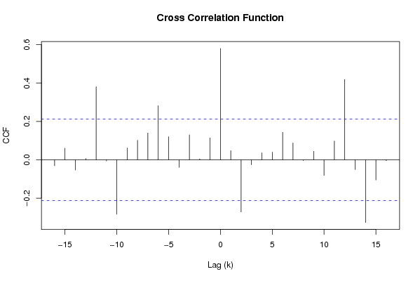
| Title produced by software | Cross Correlation Function | ||||||||||||||||||||||||||||||||||||||||||||||||||||||||||||||||||||||||||||||||||||||||||||||||||||||||||||||||||||||||||||||||||||||||||||||||||||||||||||||||||||||||||||||||||||||||||||||||
| Date of computation | Tue, 02 Dec 2008 06:18:05 -0700 | ||||||||||||||||||||||||||||||||||||||||||||||||||||||||||||||||||||||||||||||||||||||||||||||||||||||||||||||||||||||||||||||||||||||||||||||||||||||||||||||||||||||||||||||||||||||||||||||||
| Cite this page as follows | Statistical Computations at FreeStatistics.org, Office for Research Development and Education, URL https://freestatistics.org/blog/index.php?v=date/2008/Dec/02/t122822410723q0bd7ukwt143p.htm/, Retrieved Wed, 17 Sep 2025 15:04:01 +0000 | ||||||||||||||||||||||||||||||||||||||||||||||||||||||||||||||||||||||||||||||||||||||||||||||||||||||||||||||||||||||||||||||||||||||||||||||||||||||||||||||||||||||||||||||||||||||||||||||||
| Statistical Computations at FreeStatistics.org, Office for Research Development and Education, URL https://freestatistics.org/blog/index.php?pk=27739, Retrieved Wed, 17 Sep 2025 15:04:01 +0000 | |||||||||||||||||||||||||||||||||||||||||||||||||||||||||||||||||||||||||||||||||||||||||||||||||||||||||||||||||||||||||||||||||||||||||||||||||||||||||||||||||||||||||||||||||||||||||||||||||
| QR Codes: | |||||||||||||||||||||||||||||||||||||||||||||||||||||||||||||||||||||||||||||||||||||||||||||||||||||||||||||||||||||||||||||||||||||||||||||||||||||||||||||||||||||||||||||||||||||||||||||||||
|
| |||||||||||||||||||||||||||||||||||||||||||||||||||||||||||||||||||||||||||||||||||||||||||||||||||||||||||||||||||||||||||||||||||||||||||||||||||||||||||||||||||||||||||||||||||||||||||||||||
| Original text written by user: | |||||||||||||||||||||||||||||||||||||||||||||||||||||||||||||||||||||||||||||||||||||||||||||||||||||||||||||||||||||||||||||||||||||||||||||||||||||||||||||||||||||||||||||||||||||||||||||||||
| IsPrivate? | No (this computation is public) | ||||||||||||||||||||||||||||||||||||||||||||||||||||||||||||||||||||||||||||||||||||||||||||||||||||||||||||||||||||||||||||||||||||||||||||||||||||||||||||||||||||||||||||||||||||||||||||||||
| User-defined keywords | |||||||||||||||||||||||||||||||||||||||||||||||||||||||||||||||||||||||||||||||||||||||||||||||||||||||||||||||||||||||||||||||||||||||||||||||||||||||||||||||||||||||||||||||||||||||||||||||||
| Estimated Impact | 408 | ||||||||||||||||||||||||||||||||||||||||||||||||||||||||||||||||||||||||||||||||||||||||||||||||||||||||||||||||||||||||||||||||||||||||||||||||||||||||||||||||||||||||||||||||||||||||||||||||
Tree of Dependent Computations | |||||||||||||||||||||||||||||||||||||||||||||||||||||||||||||||||||||||||||||||||||||||||||||||||||||||||||||||||||||||||||||||||||||||||||||||||||||||||||||||||||||||||||||||||||||||||||||||||
| Family? (F = Feedback message, R = changed R code, M = changed R Module, P = changed Parameters, D = changed Data) | |||||||||||||||||||||||||||||||||||||||||||||||||||||||||||||||||||||||||||||||||||||||||||||||||||||||||||||||||||||||||||||||||||||||||||||||||||||||||||||||||||||||||||||||||||||||||||||||||
| F [Univariate Data Series] [Airline data] [2007-10-18 09:58:47] [42daae401fd3def69a25014f2252b4c2] F RMPD [Spectral Analysis] [airline data] [2008-12-02 12:35:12] [0e5eff269cdcaf8789c45b6ee36b0c3d] F RMPD [Cross Correlation Function] [airline data] [2008-12-02 13:18:05] [35c75b0726318bf2908e4a56ed2df1a9] [Current] F P [Cross Correlation Function] [airline data] [2008-12-02 13:46:07] [0e5eff269cdcaf8789c45b6ee36b0c3d] - RMPD [Bivariate Kernel Density Estimation] [paper] [2008-12-02 14:12:36] [0e5eff269cdcaf8789c45b6ee36b0c3d] - RMPD [Trivariate Scatterplots] [trivariate scatte...] [2008-12-02 14:28:20] [0e5eff269cdcaf8789c45b6ee36b0c3d] - RMPD [Univariate Data Series] [paper] [2008-12-02 14:39:06] [0e5eff269cdcaf8789c45b6ee36b0c3d] - RMPD [Univariate Data Series] [paper] [2008-12-02 14:41:39] [0e5eff269cdcaf8789c45b6ee36b0c3d] - RMPD [(Partial) Autocorrelation Function] [paper] [2008-12-02 14:51:55] [0e5eff269cdcaf8789c45b6ee36b0c3d] - P [(Partial) Autocorrelation Function] [acf] [2008-12-09 12:52:58] [a4602103a5e123497aa555277d0e627b] - P [(Partial) Autocorrelation Function] [acf] [2008-12-09 12:56:04] [a4602103a5e123497aa555277d0e627b] - P [(Partial) Autocorrelation Function] [acf] [2008-12-09 12:58:07] [a4602103a5e123497aa555277d0e627b] - RMPD [Variance Reduction Matrix] [vrm] [2008-12-09 14:08:41] [a4602103a5e123497aa555277d0e627b] - RMPD [Spectral Analysis] [SA] [2008-12-09 14:10:16] [a4602103a5e123497aa555277d0e627b] - RMPD [Spectral Analysis] [SA] [2008-12-09 14:12:05] [a4602103a5e123497aa555277d0e627b] - P [Spectral Analysis] [fdqsdf] [2008-12-15 14:34:13] [5387335d8669ad018e3e2def51162329] - RMPD [Spectral Analysis] [SA] [2008-12-09 14:15:20] [a4602103a5e123497aa555277d0e627b] - RMPD [Standard Deviation-Mean Plot] [SDMP] [2008-12-09 14:18:25] [a4602103a5e123497aa555277d0e627b] - RMPD [ARIMA Backward Selection] [arma] [2008-12-09 14:24:45] [a4602103a5e123497aa555277d0e627b] - RMP [Variance Reduction Matrix] [VRM] [2008-12-09 13:01:09] [a4602103a5e123497aa555277d0e627b] - RMP [Spectral Analysis] [SA] [2008-12-09 13:03:25] [a4602103a5e123497aa555277d0e627b] - RMP [Spectral Analysis] [SA] [2008-12-09 13:06:47] [a4602103a5e123497aa555277d0e627b] - RMP [Spectral Analysis] [SA] [2008-12-09 13:08:47] [a4602103a5e123497aa555277d0e627b] - RMP [Standard Deviation-Mean Plot] [SDMP] [2008-12-09 13:12:48] [a4602103a5e123497aa555277d0e627b] - RMPD [(Partial) Autocorrelation Function] [paper] [2008-12-02 14:55:43] [0e5eff269cdcaf8789c45b6ee36b0c3d] - P [(Partial) Autocorrelation Function] [acf] [2008-12-09 13:54:35] [a4602103a5e123497aa555277d0e627b] - P [(Partial) Autocorrelation Function] [acf] [2008-12-09 13:57:45] [a4602103a5e123497aa555277d0e627b] - P [(Partial) Autocorrelation Function] [qdsf] [2008-12-15 14:17:02] [5387335d8669ad018e3e2def51162329] - P [(Partial) Autocorrelation Function] [cf] [2008-12-09 14:01:52] [a4602103a5e123497aa555277d0e627b] | |||||||||||||||||||||||||||||||||||||||||||||||||||||||||||||||||||||||||||||||||||||||||||||||||||||||||||||||||||||||||||||||||||||||||||||||||||||||||||||||||||||||||||||||||||||||||||||||||
| Feedback Forum | |||||||||||||||||||||||||||||||||||||||||||||||||||||||||||||||||||||||||||||||||||||||||||||||||||||||||||||||||||||||||||||||||||||||||||||||||||||||||||||||||||||||||||||||||||||||||||||||||
Post a new message | |||||||||||||||||||||||||||||||||||||||||||||||||||||||||||||||||||||||||||||||||||||||||||||||||||||||||||||||||||||||||||||||||||||||||||||||||||||||||||||||||||||||||||||||||||||||||||||||||
Dataset | |||||||||||||||||||||||||||||||||||||||||||||||||||||||||||||||||||||||||||||||||||||||||||||||||||||||||||||||||||||||||||||||||||||||||||||||||||||||||||||||||||||||||||||||||||||||||||||||||
| Dataseries X: | |||||||||||||||||||||||||||||||||||||||||||||||||||||||||||||||||||||||||||||||||||||||||||||||||||||||||||||||||||||||||||||||||||||||||||||||||||||||||||||||||||||||||||||||||||||||||||||||||
103.1 100.6 103.1 95.5 90.5 90.9 88.8 90.7 94.3 104.6 111.1 110.8 107.2 99.0 99.0 91.0 96.2 96.9 96.2 100.1 99.0 115.4 106.9 107.1 99.3 99.2 108.3 105.6 99.5 107.4 93.1 88.1 110.7 113.1 99.6 93.6 98.6 99.6 114.3 107.8 101.2 112.5 100.5 93.9 116.2 112.0 106.4 95.7 96.0 95.8 103.0 102.2 98.4 111.4 86.6 91.3 107.9 101.8 104.4 93.4 100.1 98.5 112.9 101.4 107.1 110.8 90.3 95.5 111.4 113.0 107.5 95.9 106.3 105.2 117.2 106.9 108.2 113.0 97.2 99.9 108.1 118.1 109.1 93.3 112.1 | |||||||||||||||||||||||||||||||||||||||||||||||||||||||||||||||||||||||||||||||||||||||||||||||||||||||||||||||||||||||||||||||||||||||||||||||||||||||||||||||||||||||||||||||||||||||||||||||||
| Dataseries Y: | |||||||||||||||||||||||||||||||||||||||||||||||||||||||||||||||||||||||||||||||||||||||||||||||||||||||||||||||||||||||||||||||||||||||||||||||||||||||||||||||||||||||||||||||||||||||||||||||||
119.5 125.0 145.0 105.3 116.9 120.1 88.9 78.4 114.6 113.3 117.0 99.6 99.4 101.9 115.2 108.5 113.8 121.0 92.2 90.2 101.5 126.6 93.9 89.8 93.4 101.5 110.4 105.9 108.4 113.9 86.1 69.4 101.2 100.5 98.0 106.6 90.1 96.9 125.9 112.0 100.0 123.9 79.8 83.4 113.6 112.9 104.0 109.9 99.0 106.3 128.9 111.1 102.9 130.0 87.0 87.5 117.6 103.4 110.8 112.6 102.5 112.4 135.6 105.1 127.7 137.0 91.0 90.5 122.4 123.3 124.3 120.0 118.1 119.0 142.7 123.6 129.6 151.6 110.4 99.2 130.5 136.2 129.7 128.0 121.6 | |||||||||||||||||||||||||||||||||||||||||||||||||||||||||||||||||||||||||||||||||||||||||||||||||||||||||||||||||||||||||||||||||||||||||||||||||||||||||||||||||||||||||||||||||||||||||||||||||
Tables (Output of Computation) | |||||||||||||||||||||||||||||||||||||||||||||||||||||||||||||||||||||||||||||||||||||||||||||||||||||||||||||||||||||||||||||||||||||||||||||||||||||||||||||||||||||||||||||||||||||||||||||||||
| |||||||||||||||||||||||||||||||||||||||||||||||||||||||||||||||||||||||||||||||||||||||||||||||||||||||||||||||||||||||||||||||||||||||||||||||||||||||||||||||||||||||||||||||||||||||||||||||||
Figures (Output of Computation) | |||||||||||||||||||||||||||||||||||||||||||||||||||||||||||||||||||||||||||||||||||||||||||||||||||||||||||||||||||||||||||||||||||||||||||||||||||||||||||||||||||||||||||||||||||||||||||||||||
Input Parameters & R Code | |||||||||||||||||||||||||||||||||||||||||||||||||||||||||||||||||||||||||||||||||||||||||||||||||||||||||||||||||||||||||||||||||||||||||||||||||||||||||||||||||||||||||||||||||||||||||||||||||
| Parameters (Session): | |||||||||||||||||||||||||||||||||||||||||||||||||||||||||||||||||||||||||||||||||||||||||||||||||||||||||||||||||||||||||||||||||||||||||||||||||||||||||||||||||||||||||||||||||||||||||||||||||
| par1 = 1 ; par2 = 0 ; par3 = 0 ; par4 = 12 ; par5 = 1 ; par6 = 0 ; par7 = 0 ; | |||||||||||||||||||||||||||||||||||||||||||||||||||||||||||||||||||||||||||||||||||||||||||||||||||||||||||||||||||||||||||||||||||||||||||||||||||||||||||||||||||||||||||||||||||||||||||||||||
| Parameters (R input): | |||||||||||||||||||||||||||||||||||||||||||||||||||||||||||||||||||||||||||||||||||||||||||||||||||||||||||||||||||||||||||||||||||||||||||||||||||||||||||||||||||||||||||||||||||||||||||||||||
| par1 = 1 ; par2 = 0 ; par3 = 0 ; par4 = 12 ; par5 = 1 ; par6 = 0 ; par7 = 0 ; | |||||||||||||||||||||||||||||||||||||||||||||||||||||||||||||||||||||||||||||||||||||||||||||||||||||||||||||||||||||||||||||||||||||||||||||||||||||||||||||||||||||||||||||||||||||||||||||||||
| R code (references can be found in the software module): | |||||||||||||||||||||||||||||||||||||||||||||||||||||||||||||||||||||||||||||||||||||||||||||||||||||||||||||||||||||||||||||||||||||||||||||||||||||||||||||||||||||||||||||||||||||||||||||||||
par1 <- as.numeric(par1) | |||||||||||||||||||||||||||||||||||||||||||||||||||||||||||||||||||||||||||||||||||||||||||||||||||||||||||||||||||||||||||||||||||||||||||||||||||||||||||||||||||||||||||||||||||||||||||||||||