Repository of Reproducible Computations

Free Statistics

of Irreproducible Research!

Author's title

Author

*Unverified author*

R Software Module

rwasp_decompose.wasp

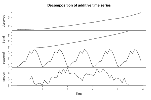
Title produced by software

Classical Decomposition

Date of computation

Fri, 25 Nov 2016 12:38:35 +0000

Cite this page as follows

Statistical Computations at FreeStatistics.org, Office for Research Development and Education, URL https://freestatistics.org/blog/index.php?v=date/2016/Nov/25/t1480077569maflitq8hjuzmmu.htm/, Retrieved Thu, 16 May 2024 02:38:03 +0200

Statistical Computations at FreeStatistics.org, Office for Research Development and Education, URL https://freestatistics.org/blog/index.php?pk=, Retrieved Thu, 16 May 2024 02:38:03 +0200

QR Codes:

Paste this QR Code to cite your computation.

Original text written by user:

IsPrivate?

No (this computation is public)

User-defined keywords

Estimated Impact

Dataseries X:

Download CSV

Histogram

Boxplots

Summary of computational transaction
Raw Input	view raw input (R code)
Raw Output	view raw output of R engine
Computing time	2 seconds
R Server	'Gwilym Jenkins' @ jenkins.wessa.net

\begin{tabular}{lllllllll}
\hline
Summary of computational transaction \tabularnewline
Raw Input & view raw input (R code)  \tabularnewline
Raw Output & view raw output of R engine  \tabularnewline
Computing time & 2 seconds \tabularnewline
R Server & 'Gwilym Jenkins' @ jenkins.wessa.net \tabularnewline
\hline
\end{tabular}
%Source: https://freestatistics.org/blog/index.php?pk=&T=0

[TABLE]
[ROW][C]Summary of computational transaction[/C][/ROW]
[ROW][C]Raw Input[/C][C]view raw input (R code) [/C][/ROW]
[ROW][C]Raw Output[/C][C]view raw output of R engine [/C][/ROW]
[ROW][C]Computing time[/C][C]2 seconds[/C][/ROW]
[ROW][C]R Server[/C][C]'Gwilym Jenkins' @ jenkins.wessa.net[/C][/ROW]
[/TABLE]
Source: https://freestatistics.org/blog/index.php?pk=&T=0

Globally Unique Identifier (entire table): ba.freestatistics.org/blog/index.php?pk=&T=0

As an alternative you can also use a QR Code:

The GUIDs for individual cells are displayed in the table below:

Summary of computational transaction
Raw Input	view raw input (R code)
Raw Output	view raw output of R engine
Computing time	2 seconds
R Server	'Gwilym Jenkins' @ jenkins.wessa.net

Classical Decomposition by Moving Averages
t	Observations	Fit	Trend	Seasonal	Random
1	103.75	NA	NA	-0.311024	NA
2	103.89	NA	NA	-0.286128	NA
3	104.01	NA	NA	-0.198628	NA
4	104.28	NA	NA	-0.131962	NA
5	104.34	NA	NA	-0.11592	NA
6	104.48	NA	NA	0.0615799	NA
7	104.56	104.767	104.523	0.24408	-0.207413
8	104.71	104.815	104.648	0.16783	-0.10533
9	104.79	105.114	104.8	0.314809	-0.324392
10	104.87	105.235	104.972	0.263038	-0.365122
11	104.95	105.286	105.179	0.107101	-0.335851
12	105	105.321	105.436	-0.114774	-0.321476
13	105.05	105.433	105.744	-0.311024	-0.383142
14	105.57	105.805	106.091	-0.286128	-0.235122
15	105.98	106.289	106.488	-0.198628	-0.309288
16	106.45	106.803	106.935	-0.131962	-0.352622
17	107.13	107.301	107.417	-0.11592	-0.170747
18	107.87	107.989	107.928	0.0615799	-0.119497
19	108.56	108.711	108.467	0.24408	-0.151163
20	109.04	109.19	109.022	0.16783	-0.149913
21	109.98	109.9	109.585	0.314809	0.080191
22	110.4	110.431	110.168	0.263038	-0.0309549
23	110.99	110.861	110.754	0.107101	0.128733
24	111.23	111.219	111.334	-0.114774	0.0110243
25	111.76	111.603	111.914	-0.311024	0.156858
26	112.18	112.211	112.497	-0.286128	-0.0309549
27	112.88	112.881	113.08	-0.198628	-0.00137153
28	113.54	113.542	113.674	-0.131962	-0.00178819
29	114.11	114.157	114.273	-0.11592	-0.0469965
30	114.8	114.939	114.877	0.0615799	-0.138663
31	115.56	115.731	115.487	0.24408	-0.171163
32	116.03	116.276	116.108	0.16783	-0.246163
33	116.98	117.07	116.755	0.314809	-0.089809
34	117.65	117.674	117.411	0.263038	-0.0238715
35	118.12	118.179	118.072	0.107101	-0.059184
36	118.6	118.636	118.751	-0.114774	-0.036059
37	119.03	119.131	119.442	-0.311024	-0.100642
38	119.82	119.853	120.139	-0.286128	-0.0326215
39	120.76	120.631	120.83	-0.198628	0.128628
40	121.4	121.381	121.513	-0.131962	0.0186285
41	122.12	122.082	122.198	-0.11592	0.0375868
42	123.08	122.949	122.887	0.0615799	0.131337
43	123.86	123.83	123.586	0.24408	0.0296701
44	124.46	124.459	124.291	0.16783	0.00133681
45	125.14	125.306	124.991	0.314809	-0.166059
46	125.89	125.97	125.707	0.263038	-0.0801215
47	126.32	126.554	126.447	0.107101	-0.233767
48	126.93	127.084	127.198	-0.114774	-0.153559
49	127.48	127.653	127.964	-0.311024	-0.173142
50	128.28	128.481	128.767	-0.286128	-0.201372
51	129.11	129.428	129.627	-0.198628	-0.318038
52	130.23	130.394	130.526	-0.131962	-0.164288
53	131.04	131.36	131.476	-0.11592	-0.319913
54	132.2	132.573	132.512	0.0615799	-0.373247
55	133.12	NA	NA	0.24408	NA
56	134.48	NA	NA	0.16783	NA
57	135.74	NA	NA	0.314809	NA
58	136.88	NA	NA	0.263038	NA
59	138.12	NA	NA	0.107101	NA
60	139.99	NA	NA	-0.114774	NA

\begin{tabular}{lllllllll}
\hline
Classical Decomposition by Moving Averages \tabularnewline
t & Observations & Fit & Trend & Seasonal & Random \tabularnewline
1 & 103.75 & NA & NA & -0.311024 & NA \tabularnewline
2 & 103.89 & NA & NA & -0.286128 & NA \tabularnewline
3 & 104.01 & NA & NA & -0.198628 & NA \tabularnewline
4 & 104.28 & NA & NA & -0.131962 & NA \tabularnewline
5 & 104.34 & NA & NA & -0.11592 & NA \tabularnewline
6 & 104.48 & NA & NA & 0.0615799 & NA \tabularnewline
7 & 104.56 & 104.767 & 104.523 & 0.24408 & -0.207413 \tabularnewline
8 & 104.71 & 104.815 & 104.648 & 0.16783 & -0.10533 \tabularnewline
9 & 104.79 & 105.114 & 104.8 & 0.314809 & -0.324392 \tabularnewline
10 & 104.87 & 105.235 & 104.972 & 0.263038 & -0.365122 \tabularnewline
11 & 104.95 & 105.286 & 105.179 & 0.107101 & -0.335851 \tabularnewline
12 & 105 & 105.321 & 105.436 & -0.114774 & -0.321476 \tabularnewline
13 & 105.05 & 105.433 & 105.744 & -0.311024 & -0.383142 \tabularnewline
14 & 105.57 & 105.805 & 106.091 & -0.286128 & -0.235122 \tabularnewline
15 & 105.98 & 106.289 & 106.488 & -0.198628 & -0.309288 \tabularnewline
16 & 106.45 & 106.803 & 106.935 & -0.131962 & -0.352622 \tabularnewline
17 & 107.13 & 107.301 & 107.417 & -0.11592 & -0.170747 \tabularnewline
18 & 107.87 & 107.989 & 107.928 & 0.0615799 & -0.119497 \tabularnewline
19 & 108.56 & 108.711 & 108.467 & 0.24408 & -0.151163 \tabularnewline
20 & 109.04 & 109.19 & 109.022 & 0.16783 & -0.149913 \tabularnewline
21 & 109.98 & 109.9 & 109.585 & 0.314809 & 0.080191 \tabularnewline
22 & 110.4 & 110.431 & 110.168 & 0.263038 & -0.0309549 \tabularnewline
23 & 110.99 & 110.861 & 110.754 & 0.107101 & 0.128733 \tabularnewline
24 & 111.23 & 111.219 & 111.334 & -0.114774 & 0.0110243 \tabularnewline
25 & 111.76 & 111.603 & 111.914 & -0.311024 & 0.156858 \tabularnewline
26 & 112.18 & 112.211 & 112.497 & -0.286128 & -0.0309549 \tabularnewline
27 & 112.88 & 112.881 & 113.08 & -0.198628 & -0.00137153 \tabularnewline
28 & 113.54 & 113.542 & 113.674 & -0.131962 & -0.00178819 \tabularnewline
29 & 114.11 & 114.157 & 114.273 & -0.11592 & -0.0469965 \tabularnewline
30 & 114.8 & 114.939 & 114.877 & 0.0615799 & -0.138663 \tabularnewline
31 & 115.56 & 115.731 & 115.487 & 0.24408 & -0.171163 \tabularnewline
32 & 116.03 & 116.276 & 116.108 & 0.16783 & -0.246163 \tabularnewline
33 & 116.98 & 117.07 & 116.755 & 0.314809 & -0.089809 \tabularnewline
34 & 117.65 & 117.674 & 117.411 & 0.263038 & -0.0238715 \tabularnewline
35 & 118.12 & 118.179 & 118.072 & 0.107101 & -0.059184 \tabularnewline
36 & 118.6 & 118.636 & 118.751 & -0.114774 & -0.036059 \tabularnewline
37 & 119.03 & 119.131 & 119.442 & -0.311024 & -0.100642 \tabularnewline
38 & 119.82 & 119.853 & 120.139 & -0.286128 & -0.0326215 \tabularnewline
39 & 120.76 & 120.631 & 120.83 & -0.198628 & 0.128628 \tabularnewline
40 & 121.4 & 121.381 & 121.513 & -0.131962 & 0.0186285 \tabularnewline
41 & 122.12 & 122.082 & 122.198 & -0.11592 & 0.0375868 \tabularnewline
42 & 123.08 & 122.949 & 122.887 & 0.0615799 & 0.131337 \tabularnewline
43 & 123.86 & 123.83 & 123.586 & 0.24408 & 0.0296701 \tabularnewline
44 & 124.46 & 124.459 & 124.291 & 0.16783 & 0.00133681 \tabularnewline
45 & 125.14 & 125.306 & 124.991 & 0.314809 & -0.166059 \tabularnewline
46 & 125.89 & 125.97 & 125.707 & 0.263038 & -0.0801215 \tabularnewline
47 & 126.32 & 126.554 & 126.447 & 0.107101 & -0.233767 \tabularnewline
48 & 126.93 & 127.084 & 127.198 & -0.114774 & -0.153559 \tabularnewline
49 & 127.48 & 127.653 & 127.964 & -0.311024 & -0.173142 \tabularnewline
50 & 128.28 & 128.481 & 128.767 & -0.286128 & -0.201372 \tabularnewline
51 & 129.11 & 129.428 & 129.627 & -0.198628 & -0.318038 \tabularnewline
52 & 130.23 & 130.394 & 130.526 & -0.131962 & -0.164288 \tabularnewline
53 & 131.04 & 131.36 & 131.476 & -0.11592 & -0.319913 \tabularnewline
54 & 132.2 & 132.573 & 132.512 & 0.0615799 & -0.373247 \tabularnewline
55 & 133.12 & NA & NA & 0.24408 & NA \tabularnewline
56 & 134.48 & NA & NA & 0.16783 & NA \tabularnewline
57 & 135.74 & NA & NA & 0.314809 & NA \tabularnewline
58 & 136.88 & NA & NA & 0.263038 & NA \tabularnewline
59 & 138.12 & NA & NA & 0.107101 & NA \tabularnewline
60 & 139.99 & NA & NA & -0.114774 & NA \tabularnewline
\hline
\end{tabular}
%Source: https://freestatistics.org/blog/index.php?pk=&T=1

[TABLE]
[ROW][C]Classical Decomposition by Moving Averages[/C][/ROW]
[ROW][C]t[/C][C]Observations[/C][C]Fit[/C][C]Trend[/C][C]Seasonal[/C][C]Random[/C][/ROW]
[ROW][C]1[/C][C]103.75[/C][C]NA[/C][C]NA[/C][C]-0.311024[/C][C]NA[/C][/ROW]
[ROW][C]2[/C][C]103.89[/C][C]NA[/C][C]NA[/C][C]-0.286128[/C][C]NA[/C][/ROW]
[ROW][C]3[/C][C]104.01[/C][C]NA[/C][C]NA[/C][C]-0.198628[/C][C]NA[/C][/ROW]
[ROW][C]4[/C][C]104.28[/C][C]NA[/C][C]NA[/C][C]-0.131962[/C][C]NA[/C][/ROW]
[ROW][C]5[/C][C]104.34[/C][C]NA[/C][C]NA[/C][C]-0.11592[/C][C]NA[/C][/ROW]
[ROW][C]6[/C][C]104.48[/C][C]NA[/C][C]NA[/C][C]0.0615799[/C][C]NA[/C][/ROW]
[ROW][C]7[/C][C]104.56[/C][C]104.767[/C][C]104.523[/C][C]0.24408[/C][C]-0.207413[/C][/ROW]
[ROW][C]8[/C][C]104.71[/C][C]104.815[/C][C]104.648[/C][C]0.16783[/C][C]-0.10533[/C][/ROW]
[ROW][C]9[/C][C]104.79[/C][C]105.114[/C][C]104.8[/C][C]0.314809[/C][C]-0.324392[/C][/ROW]
[ROW][C]10[/C][C]104.87[/C][C]105.235[/C][C]104.972[/C][C]0.263038[/C][C]-0.365122[/C][/ROW]
[ROW][C]11[/C][C]104.95[/C][C]105.286[/C][C]105.179[/C][C]0.107101[/C][C]-0.335851[/C][/ROW]
[ROW][C]12[/C][C]105[/C][C]105.321[/C][C]105.436[/C][C]-0.114774[/C][C]-0.321476[/C][/ROW]
[ROW][C]13[/C][C]105.05[/C][C]105.433[/C][C]105.744[/C][C]-0.311024[/C][C]-0.383142[/C][/ROW]
[ROW][C]14[/C][C]105.57[/C][C]105.805[/C][C]106.091[/C][C]-0.286128[/C][C]-0.235122[/C][/ROW]
[ROW][C]15[/C][C]105.98[/C][C]106.289[/C][C]106.488[/C][C]-0.198628[/C][C]-0.309288[/C][/ROW]
[ROW][C]16[/C][C]106.45[/C][C]106.803[/C][C]106.935[/C][C]-0.131962[/C][C]-0.352622[/C][/ROW]
[ROW][C]17[/C][C]107.13[/C][C]107.301[/C][C]107.417[/C][C]-0.11592[/C][C]-0.170747[/C][/ROW]
[ROW][C]18[/C][C]107.87[/C][C]107.989[/C][C]107.928[/C][C]0.0615799[/C][C]-0.119497[/C][/ROW]
[ROW][C]19[/C][C]108.56[/C][C]108.711[/C][C]108.467[/C][C]0.24408[/C][C]-0.151163[/C][/ROW]
[ROW][C]20[/C][C]109.04[/C][C]109.19[/C][C]109.022[/C][C]0.16783[/C][C]-0.149913[/C][/ROW]
[ROW][C]21[/C][C]109.98[/C][C]109.9[/C][C]109.585[/C][C]0.314809[/C][C]0.080191[/C][/ROW]
[ROW][C]22[/C][C]110.4[/C][C]110.431[/C][C]110.168[/C][C]0.263038[/C][C]-0.0309549[/C][/ROW]
[ROW][C]23[/C][C]110.99[/C][C]110.861[/C][C]110.754[/C][C]0.107101[/C][C]0.128733[/C][/ROW]
[ROW][C]24[/C][C]111.23[/C][C]111.219[/C][C]111.334[/C][C]-0.114774[/C][C]0.0110243[/C][/ROW]
[ROW][C]25[/C][C]111.76[/C][C]111.603[/C][C]111.914[/C][C]-0.311024[/C][C]0.156858[/C][/ROW]
[ROW][C]26[/C][C]112.18[/C][C]112.211[/C][C]112.497[/C][C]-0.286128[/C][C]-0.0309549[/C][/ROW]
[ROW][C]27[/C][C]112.88[/C][C]112.881[/C][C]113.08[/C][C]-0.198628[/C][C]-0.00137153[/C][/ROW]
[ROW][C]28[/C][C]113.54[/C][C]113.542[/C][C]113.674[/C][C]-0.131962[/C][C]-0.00178819[/C][/ROW]
[ROW][C]29[/C][C]114.11[/C][C]114.157[/C][C]114.273[/C][C]-0.11592[/C][C]-0.0469965[/C][/ROW]
[ROW][C]30[/C][C]114.8[/C][C]114.939[/C][C]114.877[/C][C]0.0615799[/C][C]-0.138663[/C][/ROW]
[ROW][C]31[/C][C]115.56[/C][C]115.731[/C][C]115.487[/C][C]0.24408[/C][C]-0.171163[/C][/ROW]
[ROW][C]32[/C][C]116.03[/C][C]116.276[/C][C]116.108[/C][C]0.16783[/C][C]-0.246163[/C][/ROW]
[ROW][C]33[/C][C]116.98[/C][C]117.07[/C][C]116.755[/C][C]0.314809[/C][C]-0.089809[/C][/ROW]
[ROW][C]34[/C][C]117.65[/C][C]117.674[/C][C]117.411[/C][C]0.263038[/C][C]-0.0238715[/C][/ROW]
[ROW][C]35[/C][C]118.12[/C][C]118.179[/C][C]118.072[/C][C]0.107101[/C][C]-0.059184[/C][/ROW]
[ROW][C]36[/C][C]118.6[/C][C]118.636[/C][C]118.751[/C][C]-0.114774[/C][C]-0.036059[/C][/ROW]
[ROW][C]37[/C][C]119.03[/C][C]119.131[/C][C]119.442[/C][C]-0.311024[/C][C]-0.100642[/C][/ROW]
[ROW][C]38[/C][C]119.82[/C][C]119.853[/C][C]120.139[/C][C]-0.286128[/C][C]-0.0326215[/C][/ROW]
[ROW][C]39[/C][C]120.76[/C][C]120.631[/C][C]120.83[/C][C]-0.198628[/C][C]0.128628[/C][/ROW]
[ROW][C]40[/C][C]121.4[/C][C]121.381[/C][C]121.513[/C][C]-0.131962[/C][C]0.0186285[/C][/ROW]
[ROW][C]41[/C][C]122.12[/C][C]122.082[/C][C]122.198[/C][C]-0.11592[/C][C]0.0375868[/C][/ROW]
[ROW][C]42[/C][C]123.08[/C][C]122.949[/C][C]122.887[/C][C]0.0615799[/C][C]0.131337[/C][/ROW]
[ROW][C]43[/C][C]123.86[/C][C]123.83[/C][C]123.586[/C][C]0.24408[/C][C]0.0296701[/C][/ROW]
[ROW][C]44[/C][C]124.46[/C][C]124.459[/C][C]124.291[/C][C]0.16783[/C][C]0.00133681[/C][/ROW]
[ROW][C]45[/C][C]125.14[/C][C]125.306[/C][C]124.991[/C][C]0.314809[/C][C]-0.166059[/C][/ROW]
[ROW][C]46[/C][C]125.89[/C][C]125.97[/C][C]125.707[/C][C]0.263038[/C][C]-0.0801215[/C][/ROW]
[ROW][C]47[/C][C]126.32[/C][C]126.554[/C][C]126.447[/C][C]0.107101[/C][C]-0.233767[/C][/ROW]
[ROW][C]48[/C][C]126.93[/C][C]127.084[/C][C]127.198[/C][C]-0.114774[/C][C]-0.153559[/C][/ROW]
[ROW][C]49[/C][C]127.48[/C][C]127.653[/C][C]127.964[/C][C]-0.311024[/C][C]-0.173142[/C][/ROW]
[ROW][C]50[/C][C]128.28[/C][C]128.481[/C][C]128.767[/C][C]-0.286128[/C][C]-0.201372[/C][/ROW]
[ROW][C]51[/C][C]129.11[/C][C]129.428[/C][C]129.627[/C][C]-0.198628[/C][C]-0.318038[/C][/ROW]
[ROW][C]52[/C][C]130.23[/C][C]130.394[/C][C]130.526[/C][C]-0.131962[/C][C]-0.164288[/C][/ROW]
[ROW][C]53[/C][C]131.04[/C][C]131.36[/C][C]131.476[/C][C]-0.11592[/C][C]-0.319913[/C][/ROW]
[ROW][C]54[/C][C]132.2[/C][C]132.573[/C][C]132.512[/C][C]0.0615799[/C][C]-0.373247[/C][/ROW]
[ROW][C]55[/C][C]133.12[/C][C]NA[/C][C]NA[/C][C]0.24408[/C][C]NA[/C][/ROW]
[ROW][C]56[/C][C]134.48[/C][C]NA[/C][C]NA[/C][C]0.16783[/C][C]NA[/C][/ROW]
[ROW][C]57[/C][C]135.74[/C][C]NA[/C][C]NA[/C][C]0.314809[/C][C]NA[/C][/ROW]
[ROW][C]58[/C][C]136.88[/C][C]NA[/C][C]NA[/C][C]0.263038[/C][C]NA[/C][/ROW]
[ROW][C]59[/C][C]138.12[/C][C]NA[/C][C]NA[/C][C]0.107101[/C][C]NA[/C][/ROW]
[ROW][C]60[/C][C]139.99[/C][C]NA[/C][C]NA[/C][C]-0.114774[/C][C]NA[/C][/ROW]
[/TABLE]
Source: https://freestatistics.org/blog/index.php?pk=&T=1

Globally Unique Identifier (entire table): ba.freestatistics.org/blog/index.php?pk=&T=1

As an alternative you can also use a QR Code:

The GUIDs for individual cells are displayed in the table below:

Classical Decomposition by Moving Averages
t	Observations	Fit	Trend	Seasonal	Random
1	103.75	NA	NA	-0.311024	NA
2	103.89	NA	NA	-0.286128	NA
3	104.01	NA	NA	-0.198628	NA
4	104.28	NA	NA	-0.131962	NA
5	104.34	NA	NA	-0.11592	NA
6	104.48	NA	NA	0.0615799	NA
7	104.56	104.767	104.523	0.24408	-0.207413
8	104.71	104.815	104.648	0.16783	-0.10533
9	104.79	105.114	104.8	0.314809	-0.324392
10	104.87	105.235	104.972	0.263038	-0.365122
11	104.95	105.286	105.179	0.107101	-0.335851
12	105	105.321	105.436	-0.114774	-0.321476
13	105.05	105.433	105.744	-0.311024	-0.383142
14	105.57	105.805	106.091	-0.286128	-0.235122
15	105.98	106.289	106.488	-0.198628	-0.309288
16	106.45	106.803	106.935	-0.131962	-0.352622
17	107.13	107.301	107.417	-0.11592	-0.170747
18	107.87	107.989	107.928	0.0615799	-0.119497
19	108.56	108.711	108.467	0.24408	-0.151163
20	109.04	109.19	109.022	0.16783	-0.149913
21	109.98	109.9	109.585	0.314809	0.080191
22	110.4	110.431	110.168	0.263038	-0.0309549
23	110.99	110.861	110.754	0.107101	0.128733
24	111.23	111.219	111.334	-0.114774	0.0110243
25	111.76	111.603	111.914	-0.311024	0.156858
26	112.18	112.211	112.497	-0.286128	-0.0309549
27	112.88	112.881	113.08	-0.198628	-0.00137153
28	113.54	113.542	113.674	-0.131962	-0.00178819
29	114.11	114.157	114.273	-0.11592	-0.0469965
30	114.8	114.939	114.877	0.0615799	-0.138663
31	115.56	115.731	115.487	0.24408	-0.171163
32	116.03	116.276	116.108	0.16783	-0.246163
33	116.98	117.07	116.755	0.314809	-0.089809
34	117.65	117.674	117.411	0.263038	-0.0238715
35	118.12	118.179	118.072	0.107101	-0.059184
36	118.6	118.636	118.751	-0.114774	-0.036059
37	119.03	119.131	119.442	-0.311024	-0.100642
38	119.82	119.853	120.139	-0.286128	-0.0326215
39	120.76	120.631	120.83	-0.198628	0.128628
40	121.4	121.381	121.513	-0.131962	0.0186285
41	122.12	122.082	122.198	-0.11592	0.0375868
42	123.08	122.949	122.887	0.0615799	0.131337
43	123.86	123.83	123.586	0.24408	0.0296701
44	124.46	124.459	124.291	0.16783	0.00133681
45	125.14	125.306	124.991	0.314809	-0.166059
46	125.89	125.97	125.707	0.263038	-0.0801215
47	126.32	126.554	126.447	0.107101	-0.233767
48	126.93	127.084	127.198	-0.114774	-0.153559
49	127.48	127.653	127.964	-0.311024	-0.173142
50	128.28	128.481	128.767	-0.286128	-0.201372
51	129.11	129.428	129.627	-0.198628	-0.318038
52	130.23	130.394	130.526	-0.131962	-0.164288
53	131.04	131.36	131.476	-0.11592	-0.319913
54	132.2	132.573	132.512	0.0615799	-0.373247
55	133.12	NA	NA	0.24408	NA
56	134.48	NA	NA	0.16783	NA
57	135.74	NA	NA	0.314809	NA
58	136.88	NA	NA	0.263038	NA
59	138.12	NA	NA	0.107101	NA
60	139.99	NA	NA	-0.114774	NA

Figure 1

PNG link

Postscript link

PDF link

Figure 2

PNG link

Postscript link

PDF link

Figure 3

PNG link

Postscript link

PDF link

Figure 4

PNG link

Postscript link

PDF link

Parameters (Session):

par1 = additive ; par2 = 12 ;

Parameters (R input):

par1 = additive ; par2 = 12 ;

R code (references can be found in the software module):

par2 <- as.numeric(par2)
x <- ts(x,freq=par2)
m <- decompose(x,type=par1)
m$figure
bitmap(file='test1.png')
plot(m)
dev.off()
mylagmax <- length(x)/2
bitmap(file='test2.png')
op <- par(mfrow = c(2,2))
acf(as.numeric(x),lag.max = mylagmax,main='Observed')
acf(as.numeric(m$trend),na.action=na.pass,lag.max = mylagmax,main='Trend')
acf(as.numeric(m$seasonal),na.action=na.pass,lag.max = mylagmax,main='Seasonal')
acf(as.numeric(m$random),na.action=na.pass,lag.max = mylagmax,main='Random')
par(op)
dev.off()
bitmap(file='test3.png')
op <- par(mfrow = c(2,2))
spectrum(as.numeric(x),main='Observed')
spectrum(as.numeric(m$trend[!is.na(m$trend)]),main='Trend')
spectrum(as.numeric(m$seasonal[!is.na(m$seasonal)]),main='Seasonal')
spectrum(as.numeric(m$random[!is.na(m$random)]),main='Random')
par(op)
dev.off()
bitmap(file='test4.png')
op <- par(mfrow = c(2,2))
cpgram(as.numeric(x),main='Observed')
cpgram(as.numeric(m$trend[!is.na(m$trend)]),main='Trend')
cpgram(as.numeric(m$seasonal[!is.na(m$seasonal)]),main='Seasonal')
cpgram(as.numeric(m$random[!is.na(m$random)]),main='Random')
par(op)
dev.off()
load(file='createtable')
a<-table.start()
a<-table.row.start(a)
a<-table.element(a,'Classical Decomposition by Moving Averages',6,TRUE)
a<-table.row.end(a)
a<-table.row.start(a)
a<-table.element(a,'t',header=TRUE)
a<-table.element(a,'Observations',header=TRUE)
a<-table.element(a,'Fit',header=TRUE)
a<-table.element(a,'Trend',header=TRUE)
a<-table.element(a,'Seasonal',header=TRUE)
a<-table.element(a,'Random',header=TRUE)
a<-table.row.end(a)
for (i in 1:length(m$trend)) {
a<-table.row.start(a)
a<-table.element(a,i,header=TRUE)
a<-table.element(a,x[i])
if (par1 == 'additive') a<-table.element(a,signif(m$trend[i]+m$seasonal[i],6)) else a<-table.element(a,signif(m$trend[i]*m$seasonal[i],6))
a<-table.element(a,signif(m$trend[i],6))
a<-table.element(a,signif(m$seasonal[i],6))
a<-table.element(a,signif(m$random[i],6))
a<-table.row.end(a)
}
a<-table.end(a)
table.save(a,file='mytable.tab')

Free Statistics

Description of Statistical Computation

Tree of Dependent Computations

Dataset

Tables (Output of Computation)

Figures (Output of Computation)

Input Parameters & R Code