Repository of Reproducible Computations

Free Statistics

of Irreproducible Research!

Author's title

Author

*Unverified author*

R Software Module

rwasp_decompose.wasp

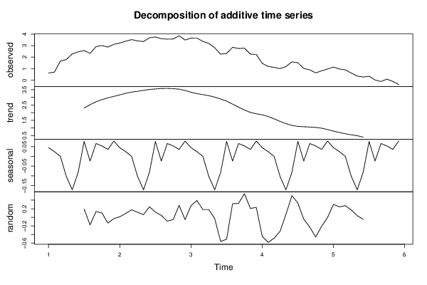
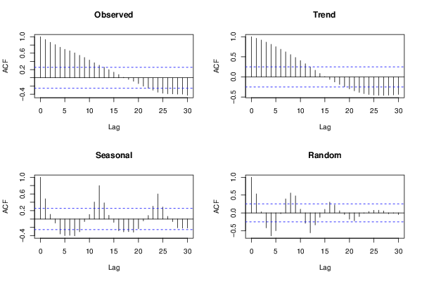
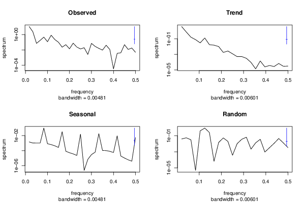
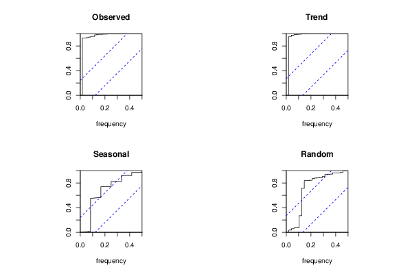
Title produced by software

Classical Decomposition

Date of computation

Sun, 29 Nov 2015 09:08:44 +0000

Cite this page as follows

Statistical Computations at FreeStatistics.org, Office for Research Development and Education, URL https://freestatistics.org/blog/index.php?v=date/2015/Nov/29/t1448788150zs67jf8ejibn85g.htm/, Retrieved Wed, 15 May 2024 04:53:47 +0000

Statistical Computations at FreeStatistics.org, Office for Research Development and Education, URL https://freestatistics.org/blog/index.php?pk=284399, Retrieved Wed, 15 May 2024 04:53:47 +0000

QR Codes:

Paste this QR Code to cite your computation.

Original text written by user:

IsPrivate?

No (this computation is public)

User-defined keywords

Estimated Impact

129

Family? (F = Feedback message, R = changed R code, M = changed R Module, P = changed Parameters, D = changed Data)

-       [Classical Decomposition] [] [2015-11-29 09:08:44] [935c69a10ec4a64678755fcf1ddf3064] [Current]

Feedback Forum

Post a new message

Dataseries X:

Download CSV

Histogram

Boxplots

0,62
0,7
1,65
1,79
2,28
2,46
2,57
2,32
2,91
3,01
2,87
3,11
3,22
3,38
3,52
3,41
3,35
3,68
3,75
3,6
3,56
3,57
3,85
3,48
3,65
3,66
3,36
3,19
2,81
2,25
2,32
2,85
2,75
2,78
2,26
2,23
1,46
1,19
1,11
1
1,18
1,59
1,51
1,01
0,9
0,63
0,81
0,97
1,14
0,97
0,89
0,62
0,36
0,27
0,34
0,02
-0,12
0,09
-0,11
-0,38

Summary of computational transaction
Raw Input	view raw input (R code)
Raw Output	view raw output of R engine
Computing time	2 seconds
R Server	'Sir Maurice George Kendall' @ kendall.wessa.net

\begin{tabular}{lllllllll}
\hline
Summary of computational transaction \tabularnewline
Raw Input & view raw input (R code)  \tabularnewline
Raw Output & view raw output of R engine  \tabularnewline
Computing time & 2 seconds \tabularnewline
R Server & 'Sir Maurice George Kendall' @ kendall.wessa.net \tabularnewline
\hline
\end{tabular}
%Source: https://freestatistics.org/blog/index.php?pk=284399&T=0

[TABLE]
[ROW][C]Summary of computational transaction[/C][/ROW]
[ROW][C]Raw Input[/C][C]view raw input (R code) [/C][/ROW]
[ROW][C]Raw Output[/C][C]view raw output of R engine [/C][/ROW]
[ROW][C]Computing time[/C][C]2 seconds[/C][/ROW]
[ROW][C]R Server[/C][C]'Sir Maurice George Kendall' @ kendall.wessa.net[/C][/ROW]
[/TABLE]
Source: https://freestatistics.org/blog/index.php?pk=284399&T=0

Globally Unique Identifier (entire table): ba.freestatistics.org/blog/index.php?pk=284399&T=0

As an alternative you can also use a QR Code:

The GUIDs for individual cells are displayed in the table below:

Summary of computational transaction
Raw Input	view raw input (R code)
Raw Output	view raw output of R engine
Computing time	2 seconds
R Server	'Sir Maurice George Kendall' @ kendall.wessa.net

Classical Decomposition by Moving Averages
t	Observations	Fit	Trend	Seasonal	Random
1	0.62	NA	NA	0.0447569	NA
2	0.7	NA	NA	0.0244444	NA
3	1.65	NA	NA	-3.47222e-05	NA
4	1.79	NA	NA	-0.103056	NA
5	2.28	NA	NA	-0.171597	NA
6	2.46	NA	NA	-0.0817014	NA
7	2.57	2.3759	2.29917	0.0767361	0.194097
8	2.32	2.49517	2.51917	-0.0239931	-0.175174
9	2.91	2.77486	2.70875	0.0661111	0.135139
10	3.01	2.90788	2.85417	0.0537153	0.102118
11	2.87	3.00215	2.96625	0.0359028	-0.132153
12	3.11	3.14038	3.06167	0.0787153	-0.0303819
13	3.22	3.20642	3.16167	0.0447569	0.0135764
14	3.38	3.28861	3.26417	0.0244444	0.0913889
15	3.52	3.34455	3.34458	-3.47222e-05	0.175451
16	3.41	3.29194	3.395	-0.103056	0.118056
17	3.35	3.28757	3.45917	-0.171597	0.0624306
18	3.68	3.43372	3.51542	-0.0817014	0.246285
19	3.75	3.62549	3.54875	0.0767361	0.124514
20	3.6	3.55434	3.57833	-0.0239931	0.0456597
21	3.56	3.64944	3.58333	0.0661111	-0.0894444
22	3.57	3.62122	3.5675	0.0537153	-0.0512153
23	3.85	3.57174	3.53583	0.0359028	0.278264
24	3.48	3.53247	3.45375	0.0787153	-0.0524653
25	3.65	3.37934	3.33458	0.0447569	0.27066
26	3.66	3.26819	3.24375	0.0244444	0.391806
27	3.36	3.17872	3.17875	-3.47222e-05	0.181285
28	3.19	3.00903	3.11208	-0.103056	0.180972
29	2.81	2.84132	3.01292	-0.171597	-0.0313194
30	2.25	2.81288	2.89458	-0.0817014	-0.562882
31	2.32	2.82799	2.75125	0.0767361	-0.507986
32	2.85	2.53309	2.55708	-0.0239931	0.31691
33	2.75	2.42653	2.36042	0.0661111	0.323472
34	2.78	2.22913	2.17542	0.0537153	0.550868
35	2.26	2.05215	2.01625	0.0359028	0.207847
36	2.23	1.99955	1.92083	0.0787153	0.230451
37	1.46	1.90434	1.85958	0.0447569	-0.44434
38	1.19	1.77361	1.74917	0.0244444	-0.583611
39	1.11	1.59538	1.59542	-3.47222e-05	-0.485382
40	1	1.32569	1.42875	-0.103056	-0.325694
41	1.18	1.10715	1.27875	-0.171597	0.0728472
42	1.59	1.08413	1.16583	-0.0817014	0.505868
43	1.51	1.17674	1.1	0.0767361	0.333264
44	1.01	1.05351	1.0775	-0.0239931	-0.0435069
45	0.9	1.12528	1.05917	0.0661111	-0.225278
46	0.63	1.08788	1.03417	0.0537153	-0.457882
47	0.81	1.02007	0.984167	0.0359028	-0.210069
48	0.97	0.973715	0.895	0.0787153	-0.00371528
49	1.14	0.836007	0.79125	0.0447569	0.303993
50	0.97	0.725694	0.70125	0.0244444	0.244306
51	0.89	0.617465	0.6175	-3.47222e-05	0.272535
52	0.62	0.449444	0.5525	-0.103056	0.170556
53	0.36	0.320069	0.491667	-0.171597	0.0399306
54	0.27	0.315382	0.397083	-0.0817014	-0.0453819
55	0.34	NA	NA	0.0767361	NA
56	0.02	NA	NA	-0.0239931	NA
57	-0.12	NA	NA	0.0661111	NA
58	0.09	NA	NA	0.0537153	NA
59	-0.11	NA	NA	0.0359028	NA
60	-0.38	NA	NA	0.0787153	NA

\begin{tabular}{lllllllll}
\hline
Classical Decomposition by Moving Averages \tabularnewline
t & Observations & Fit & Trend & Seasonal & Random \tabularnewline
1 & 0.62 & NA & NA & 0.0447569 & NA \tabularnewline
2 & 0.7 & NA & NA & 0.0244444 & NA \tabularnewline
3 & 1.65 & NA & NA & -3.47222e-05 & NA \tabularnewline
4 & 1.79 & NA & NA & -0.103056 & NA \tabularnewline
5 & 2.28 & NA & NA & -0.171597 & NA \tabularnewline
6 & 2.46 & NA & NA & -0.0817014 & NA \tabularnewline
7 & 2.57 & 2.3759 & 2.29917 & 0.0767361 & 0.194097 \tabularnewline
8 & 2.32 & 2.49517 & 2.51917 & -0.0239931 & -0.175174 \tabularnewline
9 & 2.91 & 2.77486 & 2.70875 & 0.0661111 & 0.135139 \tabularnewline
10 & 3.01 & 2.90788 & 2.85417 & 0.0537153 & 0.102118 \tabularnewline
11 & 2.87 & 3.00215 & 2.96625 & 0.0359028 & -0.132153 \tabularnewline
12 & 3.11 & 3.14038 & 3.06167 & 0.0787153 & -0.0303819 \tabularnewline
13 & 3.22 & 3.20642 & 3.16167 & 0.0447569 & 0.0135764 \tabularnewline
14 & 3.38 & 3.28861 & 3.26417 & 0.0244444 & 0.0913889 \tabularnewline
15 & 3.52 & 3.34455 & 3.34458 & -3.47222e-05 & 0.175451 \tabularnewline
16 & 3.41 & 3.29194 & 3.395 & -0.103056 & 0.118056 \tabularnewline
17 & 3.35 & 3.28757 & 3.45917 & -0.171597 & 0.0624306 \tabularnewline
18 & 3.68 & 3.43372 & 3.51542 & -0.0817014 & 0.246285 \tabularnewline
19 & 3.75 & 3.62549 & 3.54875 & 0.0767361 & 0.124514 \tabularnewline
20 & 3.6 & 3.55434 & 3.57833 & -0.0239931 & 0.0456597 \tabularnewline
21 & 3.56 & 3.64944 & 3.58333 & 0.0661111 & -0.0894444 \tabularnewline
22 & 3.57 & 3.62122 & 3.5675 & 0.0537153 & -0.0512153 \tabularnewline
23 & 3.85 & 3.57174 & 3.53583 & 0.0359028 & 0.278264 \tabularnewline
24 & 3.48 & 3.53247 & 3.45375 & 0.0787153 & -0.0524653 \tabularnewline
25 & 3.65 & 3.37934 & 3.33458 & 0.0447569 & 0.27066 \tabularnewline
26 & 3.66 & 3.26819 & 3.24375 & 0.0244444 & 0.391806 \tabularnewline
27 & 3.36 & 3.17872 & 3.17875 & -3.47222e-05 & 0.181285 \tabularnewline
28 & 3.19 & 3.00903 & 3.11208 & -0.103056 & 0.180972 \tabularnewline
29 & 2.81 & 2.84132 & 3.01292 & -0.171597 & -0.0313194 \tabularnewline
30 & 2.25 & 2.81288 & 2.89458 & -0.0817014 & -0.562882 \tabularnewline
31 & 2.32 & 2.82799 & 2.75125 & 0.0767361 & -0.507986 \tabularnewline
32 & 2.85 & 2.53309 & 2.55708 & -0.0239931 & 0.31691 \tabularnewline
33 & 2.75 & 2.42653 & 2.36042 & 0.0661111 & 0.323472 \tabularnewline
34 & 2.78 & 2.22913 & 2.17542 & 0.0537153 & 0.550868 \tabularnewline
35 & 2.26 & 2.05215 & 2.01625 & 0.0359028 & 0.207847 \tabularnewline
36 & 2.23 & 1.99955 & 1.92083 & 0.0787153 & 0.230451 \tabularnewline
37 & 1.46 & 1.90434 & 1.85958 & 0.0447569 & -0.44434 \tabularnewline
38 & 1.19 & 1.77361 & 1.74917 & 0.0244444 & -0.583611 \tabularnewline
39 & 1.11 & 1.59538 & 1.59542 & -3.47222e-05 & -0.485382 \tabularnewline
40 & 1 & 1.32569 & 1.42875 & -0.103056 & -0.325694 \tabularnewline
41 & 1.18 & 1.10715 & 1.27875 & -0.171597 & 0.0728472 \tabularnewline
42 & 1.59 & 1.08413 & 1.16583 & -0.0817014 & 0.505868 \tabularnewline
43 & 1.51 & 1.17674 & 1.1 & 0.0767361 & 0.333264 \tabularnewline
44 & 1.01 & 1.05351 & 1.0775 & -0.0239931 & -0.0435069 \tabularnewline
45 & 0.9 & 1.12528 & 1.05917 & 0.0661111 & -0.225278 \tabularnewline
46 & 0.63 & 1.08788 & 1.03417 & 0.0537153 & -0.457882 \tabularnewline
47 & 0.81 & 1.02007 & 0.984167 & 0.0359028 & -0.210069 \tabularnewline
48 & 0.97 & 0.973715 & 0.895 & 0.0787153 & -0.00371528 \tabularnewline
49 & 1.14 & 0.836007 & 0.79125 & 0.0447569 & 0.303993 \tabularnewline
50 & 0.97 & 0.725694 & 0.70125 & 0.0244444 & 0.244306 \tabularnewline
51 & 0.89 & 0.617465 & 0.6175 & -3.47222e-05 & 0.272535 \tabularnewline
52 & 0.62 & 0.449444 & 0.5525 & -0.103056 & 0.170556 \tabularnewline
53 & 0.36 & 0.320069 & 0.491667 & -0.171597 & 0.0399306 \tabularnewline
54 & 0.27 & 0.315382 & 0.397083 & -0.0817014 & -0.0453819 \tabularnewline
55 & 0.34 & NA & NA & 0.0767361 & NA \tabularnewline
56 & 0.02 & NA & NA & -0.0239931 & NA \tabularnewline
57 & -0.12 & NA & NA & 0.0661111 & NA \tabularnewline
58 & 0.09 & NA & NA & 0.0537153 & NA \tabularnewline
59 & -0.11 & NA & NA & 0.0359028 & NA \tabularnewline
60 & -0.38 & NA & NA & 0.0787153 & NA \tabularnewline
\hline
\end{tabular}
%Source: https://freestatistics.org/blog/index.php?pk=284399&T=1

[TABLE]
[ROW][C]Classical Decomposition by Moving Averages[/C][/ROW]
[ROW][C]t[/C][C]Observations[/C][C]Fit[/C][C]Trend[/C][C]Seasonal[/C][C]Random[/C][/ROW]
[ROW][C]1[/C][C]0.62[/C][C]NA[/C][C]NA[/C][C]0.0447569[/C][C]NA[/C][/ROW]
[ROW][C]2[/C][C]0.7[/C][C]NA[/C][C]NA[/C][C]0.0244444[/C][C]NA[/C][/ROW]
[ROW][C]3[/C][C]1.65[/C][C]NA[/C][C]NA[/C][C]-3.47222e-05[/C][C]NA[/C][/ROW]
[ROW][C]4[/C][C]1.79[/C][C]NA[/C][C]NA[/C][C]-0.103056[/C][C]NA[/C][/ROW]
[ROW][C]5[/C][C]2.28[/C][C]NA[/C][C]NA[/C][C]-0.171597[/C][C]NA[/C][/ROW]
[ROW][C]6[/C][C]2.46[/C][C]NA[/C][C]NA[/C][C]-0.0817014[/C][C]NA[/C][/ROW]
[ROW][C]7[/C][C]2.57[/C][C]2.3759[/C][C]2.29917[/C][C]0.0767361[/C][C]0.194097[/C][/ROW]
[ROW][C]8[/C][C]2.32[/C][C]2.49517[/C][C]2.51917[/C][C]-0.0239931[/C][C]-0.175174[/C][/ROW]
[ROW][C]9[/C][C]2.91[/C][C]2.77486[/C][C]2.70875[/C][C]0.0661111[/C][C]0.135139[/C][/ROW]
[ROW][C]10[/C][C]3.01[/C][C]2.90788[/C][C]2.85417[/C][C]0.0537153[/C][C]0.102118[/C][/ROW]
[ROW][C]11[/C][C]2.87[/C][C]3.00215[/C][C]2.96625[/C][C]0.0359028[/C][C]-0.132153[/C][/ROW]
[ROW][C]12[/C][C]3.11[/C][C]3.14038[/C][C]3.06167[/C][C]0.0787153[/C][C]-0.0303819[/C][/ROW]
[ROW][C]13[/C][C]3.22[/C][C]3.20642[/C][C]3.16167[/C][C]0.0447569[/C][C]0.0135764[/C][/ROW]
[ROW][C]14[/C][C]3.38[/C][C]3.28861[/C][C]3.26417[/C][C]0.0244444[/C][C]0.0913889[/C][/ROW]
[ROW][C]15[/C][C]3.52[/C][C]3.34455[/C][C]3.34458[/C][C]-3.47222e-05[/C][C]0.175451[/C][/ROW]
[ROW][C]16[/C][C]3.41[/C][C]3.29194[/C][C]3.395[/C][C]-0.103056[/C][C]0.118056[/C][/ROW]
[ROW][C]17[/C][C]3.35[/C][C]3.28757[/C][C]3.45917[/C][C]-0.171597[/C][C]0.0624306[/C][/ROW]
[ROW][C]18[/C][C]3.68[/C][C]3.43372[/C][C]3.51542[/C][C]-0.0817014[/C][C]0.246285[/C][/ROW]
[ROW][C]19[/C][C]3.75[/C][C]3.62549[/C][C]3.54875[/C][C]0.0767361[/C][C]0.124514[/C][/ROW]
[ROW][C]20[/C][C]3.6[/C][C]3.55434[/C][C]3.57833[/C][C]-0.0239931[/C][C]0.0456597[/C][/ROW]
[ROW][C]21[/C][C]3.56[/C][C]3.64944[/C][C]3.58333[/C][C]0.0661111[/C][C]-0.0894444[/C][/ROW]
[ROW][C]22[/C][C]3.57[/C][C]3.62122[/C][C]3.5675[/C][C]0.0537153[/C][C]-0.0512153[/C][/ROW]
[ROW][C]23[/C][C]3.85[/C][C]3.57174[/C][C]3.53583[/C][C]0.0359028[/C][C]0.278264[/C][/ROW]
[ROW][C]24[/C][C]3.48[/C][C]3.53247[/C][C]3.45375[/C][C]0.0787153[/C][C]-0.0524653[/C][/ROW]
[ROW][C]25[/C][C]3.65[/C][C]3.37934[/C][C]3.33458[/C][C]0.0447569[/C][C]0.27066[/C][/ROW]
[ROW][C]26[/C][C]3.66[/C][C]3.26819[/C][C]3.24375[/C][C]0.0244444[/C][C]0.391806[/C][/ROW]
[ROW][C]27[/C][C]3.36[/C][C]3.17872[/C][C]3.17875[/C][C]-3.47222e-05[/C][C]0.181285[/C][/ROW]
[ROW][C]28[/C][C]3.19[/C][C]3.00903[/C][C]3.11208[/C][C]-0.103056[/C][C]0.180972[/C][/ROW]
[ROW][C]29[/C][C]2.81[/C][C]2.84132[/C][C]3.01292[/C][C]-0.171597[/C][C]-0.0313194[/C][/ROW]
[ROW][C]30[/C][C]2.25[/C][C]2.81288[/C][C]2.89458[/C][C]-0.0817014[/C][C]-0.562882[/C][/ROW]
[ROW][C]31[/C][C]2.32[/C][C]2.82799[/C][C]2.75125[/C][C]0.0767361[/C][C]-0.507986[/C][/ROW]
[ROW][C]32[/C][C]2.85[/C][C]2.53309[/C][C]2.55708[/C][C]-0.0239931[/C][C]0.31691[/C][/ROW]
[ROW][C]33[/C][C]2.75[/C][C]2.42653[/C][C]2.36042[/C][C]0.0661111[/C][C]0.323472[/C][/ROW]
[ROW][C]34[/C][C]2.78[/C][C]2.22913[/C][C]2.17542[/C][C]0.0537153[/C][C]0.550868[/C][/ROW]
[ROW][C]35[/C][C]2.26[/C][C]2.05215[/C][C]2.01625[/C][C]0.0359028[/C][C]0.207847[/C][/ROW]
[ROW][C]36[/C][C]2.23[/C][C]1.99955[/C][C]1.92083[/C][C]0.0787153[/C][C]0.230451[/C][/ROW]
[ROW][C]37[/C][C]1.46[/C][C]1.90434[/C][C]1.85958[/C][C]0.0447569[/C][C]-0.44434[/C][/ROW]
[ROW][C]38[/C][C]1.19[/C][C]1.77361[/C][C]1.74917[/C][C]0.0244444[/C][C]-0.583611[/C][/ROW]
[ROW][C]39[/C][C]1.11[/C][C]1.59538[/C][C]1.59542[/C][C]-3.47222e-05[/C][C]-0.485382[/C][/ROW]
[ROW][C]40[/C][C]1[/C][C]1.32569[/C][C]1.42875[/C][C]-0.103056[/C][C]-0.325694[/C][/ROW]
[ROW][C]41[/C][C]1.18[/C][C]1.10715[/C][C]1.27875[/C][C]-0.171597[/C][C]0.0728472[/C][/ROW]
[ROW][C]42[/C][C]1.59[/C][C]1.08413[/C][C]1.16583[/C][C]-0.0817014[/C][C]0.505868[/C][/ROW]
[ROW][C]43[/C][C]1.51[/C][C]1.17674[/C][C]1.1[/C][C]0.0767361[/C][C]0.333264[/C][/ROW]
[ROW][C]44[/C][C]1.01[/C][C]1.05351[/C][C]1.0775[/C][C]-0.0239931[/C][C]-0.0435069[/C][/ROW]
[ROW][C]45[/C][C]0.9[/C][C]1.12528[/C][C]1.05917[/C][C]0.0661111[/C][C]-0.225278[/C][/ROW]
[ROW][C]46[/C][C]0.63[/C][C]1.08788[/C][C]1.03417[/C][C]0.0537153[/C][C]-0.457882[/C][/ROW]
[ROW][C]47[/C][C]0.81[/C][C]1.02007[/C][C]0.984167[/C][C]0.0359028[/C][C]-0.210069[/C][/ROW]
[ROW][C]48[/C][C]0.97[/C][C]0.973715[/C][C]0.895[/C][C]0.0787153[/C][C]-0.00371528[/C][/ROW]
[ROW][C]49[/C][C]1.14[/C][C]0.836007[/C][C]0.79125[/C][C]0.0447569[/C][C]0.303993[/C][/ROW]
[ROW][C]50[/C][C]0.97[/C][C]0.725694[/C][C]0.70125[/C][C]0.0244444[/C][C]0.244306[/C][/ROW]
[ROW][C]51[/C][C]0.89[/C][C]0.617465[/C][C]0.6175[/C][C]-3.47222e-05[/C][C]0.272535[/C][/ROW]
[ROW][C]52[/C][C]0.62[/C][C]0.449444[/C][C]0.5525[/C][C]-0.103056[/C][C]0.170556[/C][/ROW]
[ROW][C]53[/C][C]0.36[/C][C]0.320069[/C][C]0.491667[/C][C]-0.171597[/C][C]0.0399306[/C][/ROW]
[ROW][C]54[/C][C]0.27[/C][C]0.315382[/C][C]0.397083[/C][C]-0.0817014[/C][C]-0.0453819[/C][/ROW]
[ROW][C]55[/C][C]0.34[/C][C]NA[/C][C]NA[/C][C]0.0767361[/C][C]NA[/C][/ROW]
[ROW][C]56[/C][C]0.02[/C][C]NA[/C][C]NA[/C][C]-0.0239931[/C][C]NA[/C][/ROW]
[ROW][C]57[/C][C]-0.12[/C][C]NA[/C][C]NA[/C][C]0.0661111[/C][C]NA[/C][/ROW]
[ROW][C]58[/C][C]0.09[/C][C]NA[/C][C]NA[/C][C]0.0537153[/C][C]NA[/C][/ROW]
[ROW][C]59[/C][C]-0.11[/C][C]NA[/C][C]NA[/C][C]0.0359028[/C][C]NA[/C][/ROW]
[ROW][C]60[/C][C]-0.38[/C][C]NA[/C][C]NA[/C][C]0.0787153[/C][C]NA[/C][/ROW]
[/TABLE]
Source: https://freestatistics.org/blog/index.php?pk=284399&T=1

Globally Unique Identifier (entire table): ba.freestatistics.org/blog/index.php?pk=284399&T=1

As an alternative you can also use a QR Code:

The GUIDs for individual cells are displayed in the table below:

Classical Decomposition by Moving Averages
t	Observations	Fit	Trend	Seasonal	Random
1	0.62	NA	NA	0.0447569	NA
2	0.7	NA	NA	0.0244444	NA
3	1.65	NA	NA	-3.47222e-05	NA
4	1.79	NA	NA	-0.103056	NA
5	2.28	NA	NA	-0.171597	NA
6	2.46	NA	NA	-0.0817014	NA
7	2.57	2.3759	2.29917	0.0767361	0.194097
8	2.32	2.49517	2.51917	-0.0239931	-0.175174
9	2.91	2.77486	2.70875	0.0661111	0.135139
10	3.01	2.90788	2.85417	0.0537153	0.102118
11	2.87	3.00215	2.96625	0.0359028	-0.132153
12	3.11	3.14038	3.06167	0.0787153	-0.0303819
13	3.22	3.20642	3.16167	0.0447569	0.0135764
14	3.38	3.28861	3.26417	0.0244444	0.0913889
15	3.52	3.34455	3.34458	-3.47222e-05	0.175451
16	3.41	3.29194	3.395	-0.103056	0.118056
17	3.35	3.28757	3.45917	-0.171597	0.0624306
18	3.68	3.43372	3.51542	-0.0817014	0.246285
19	3.75	3.62549	3.54875	0.0767361	0.124514
20	3.6	3.55434	3.57833	-0.0239931	0.0456597
21	3.56	3.64944	3.58333	0.0661111	-0.0894444
22	3.57	3.62122	3.5675	0.0537153	-0.0512153
23	3.85	3.57174	3.53583	0.0359028	0.278264
24	3.48	3.53247	3.45375	0.0787153	-0.0524653
25	3.65	3.37934	3.33458	0.0447569	0.27066
26	3.66	3.26819	3.24375	0.0244444	0.391806
27	3.36	3.17872	3.17875	-3.47222e-05	0.181285
28	3.19	3.00903	3.11208	-0.103056	0.180972
29	2.81	2.84132	3.01292	-0.171597	-0.0313194
30	2.25	2.81288	2.89458	-0.0817014	-0.562882
31	2.32	2.82799	2.75125	0.0767361	-0.507986
32	2.85	2.53309	2.55708	-0.0239931	0.31691
33	2.75	2.42653	2.36042	0.0661111	0.323472
34	2.78	2.22913	2.17542	0.0537153	0.550868
35	2.26	2.05215	2.01625	0.0359028	0.207847
36	2.23	1.99955	1.92083	0.0787153	0.230451
37	1.46	1.90434	1.85958	0.0447569	-0.44434
38	1.19	1.77361	1.74917	0.0244444	-0.583611
39	1.11	1.59538	1.59542	-3.47222e-05	-0.485382
40	1	1.32569	1.42875	-0.103056	-0.325694
41	1.18	1.10715	1.27875	-0.171597	0.0728472
42	1.59	1.08413	1.16583	-0.0817014	0.505868
43	1.51	1.17674	1.1	0.0767361	0.333264
44	1.01	1.05351	1.0775	-0.0239931	-0.0435069
45	0.9	1.12528	1.05917	0.0661111	-0.225278
46	0.63	1.08788	1.03417	0.0537153	-0.457882
47	0.81	1.02007	0.984167	0.0359028	-0.210069
48	0.97	0.973715	0.895	0.0787153	-0.00371528
49	1.14	0.836007	0.79125	0.0447569	0.303993
50	0.97	0.725694	0.70125	0.0244444	0.244306
51	0.89	0.617465	0.6175	-3.47222e-05	0.272535
52	0.62	0.449444	0.5525	-0.103056	0.170556
53	0.36	0.320069	0.491667	-0.171597	0.0399306
54	0.27	0.315382	0.397083	-0.0817014	-0.0453819
55	0.34	NA	NA	0.0767361	NA
56	0.02	NA	NA	-0.0239931	NA
57	-0.12	NA	NA	0.0661111	NA
58	0.09	NA	NA	0.0537153	NA
59	-0.11	NA	NA	0.0359028	NA
60	-0.38	NA	NA	0.0787153	NA

Figure 1

PNG link

Postscript link

PDF link

Figure 2

PNG link

Postscript link

PDF link

Figure 3

PNG link

Postscript link

PDF link

Figure 4

PNG link

Postscript link

PDF link

Parameters (Session):

par1 = additive ; par2 = 12 ;

Parameters (R input):

par1 = additive ; par2 = 12 ;

R code (references can be found in the software module):

par2 <- as.numeric(par2)
x <- ts(x,freq=par2)
m <- decompose(x,type=par1)
m$figure
bitmap(file='test1.png')
plot(m)
dev.off()
mylagmax <- length(x)/2
bitmap(file='test2.png')
op <- par(mfrow = c(2,2))
acf(as.numeric(x),lag.max = mylagmax,main='Observed')
acf(as.numeric(m$trend),na.action=na.pass,lag.max = mylagmax,main='Trend')
acf(as.numeric(m$seasonal),na.action=na.pass,lag.max = mylagmax,main='Seasonal')
acf(as.numeric(m$random),na.action=na.pass,lag.max = mylagmax,main='Random')
par(op)
dev.off()
bitmap(file='test3.png')
op <- par(mfrow = c(2,2))
spectrum(as.numeric(x),main='Observed')
spectrum(as.numeric(m$trend[!is.na(m$trend)]),main='Trend')
spectrum(as.numeric(m$seasonal[!is.na(m$seasonal)]),main='Seasonal')
spectrum(as.numeric(m$random[!is.na(m$random)]),main='Random')
par(op)
dev.off()
bitmap(file='test4.png')
op <- par(mfrow = c(2,2))
cpgram(as.numeric(x),main='Observed')
cpgram(as.numeric(m$trend[!is.na(m$trend)]),main='Trend')
cpgram(as.numeric(m$seasonal[!is.na(m$seasonal)]),main='Seasonal')
cpgram(as.numeric(m$random[!is.na(m$random)]),main='Random')
par(op)
dev.off()
load(file='createtable')
a<-table.start()
a<-table.row.start(a)
a<-table.element(a,'Classical Decomposition by Moving Averages',6,TRUE)
a<-table.row.end(a)
a<-table.row.start(a)
a<-table.element(a,'t',header=TRUE)
a<-table.element(a,'Observations',header=TRUE)
a<-table.element(a,'Fit',header=TRUE)
a<-table.element(a,'Trend',header=TRUE)
a<-table.element(a,'Seasonal',header=TRUE)
a<-table.element(a,'Random',header=TRUE)
a<-table.row.end(a)
for (i in 1:length(m$trend)) {
a<-table.row.start(a)
a<-table.element(a,i,header=TRUE)
a<-table.element(a,x[i])
if (par1 == 'additive') a<-table.element(a,signif(m$trend[i]+m$seasonal[i],6)) else a<-table.element(a,signif(m$trend[i]*m$seasonal[i],6))
a<-table.element(a,signif(m$trend[i],6))
a<-table.element(a,signif(m$seasonal[i],6))
a<-table.element(a,signif(m$random[i],6))
a<-table.row.end(a)
}
a<-table.end(a)
table.save(a,file='mytable.tab')

Free Statistics

Description of Statistical Computation

Tree of Dependent Computations

Dataset

Tables (Output of Computation)

Figures (Output of Computation)

Input Parameters & R Code