Free Statistics
of Irreproducible Research!
Description of Statistical Computation | |||||||||||||||||||||
|---|---|---|---|---|---|---|---|---|---|---|---|---|---|---|---|---|---|---|---|---|---|
| Author's title | |||||||||||||||||||||
| Author | *The author of this computation has been verified* | ||||||||||||||||||||
| R Software Module | rwasp_meanplot.wasp | ||||||||||||||||||||
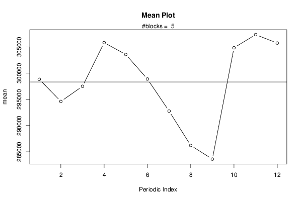
| Title produced by software | Mean Plot | ||||||||||||||||||||
| Date of computation | Sat, 28 Nov 2015 17:51:11 +0000 | ||||||||||||||||||||
| Cite this page as follows | Statistical Computations at FreeStatistics.org, Office for Research Development and Education, URL https://freestatistics.org/blog/index.php?v=date/2015/Nov/28/t1448733092yxacgcrf16rfsk6.htm/, Retrieved Mon, 13 May 2024 23:43:02 +0000 | ||||||||||||||||||||
| Statistical Computations at FreeStatistics.org, Office for Research Development and Education, URL https://freestatistics.org/blog/index.php?pk=284383, Retrieved Mon, 13 May 2024 23:43:02 +0000 | |||||||||||||||||||||
| QR Codes: | |||||||||||||||||||||
|
| |||||||||||||||||||||
| Original text written by user: | |||||||||||||||||||||
| IsPrivate? | No (this computation is public) | ||||||||||||||||||||
| User-defined keywords | |||||||||||||||||||||
| Estimated Impact | 98 | ||||||||||||||||||||
Tree of Dependent Computations | |||||||||||||||||||||
| Family? (F = Feedback message, R = changed R code, M = changed R Module, P = changed Parameters, D = changed Data) | |||||||||||||||||||||
| F [Central Tendency] [Time needed to su...] [2010-09-25 09:42:08] [b98453cac15ba1066b407e146608df68] - RMPD [Mean Plot] [Mean plot totaal ...] [2015-11-28 17:51:11] [20fcaaf1d4bc4a12bf87c6c50d624c14] [Current] - R [Mean Plot] [] [2015-12-17 20:00:08] [22b6f4a061c8797aa483199554a73d13] | |||||||||||||||||||||
| Feedback Forum | |||||||||||||||||||||
Post a new message | |||||||||||||||||||||
Dataset | |||||||||||||||||||||
| Dataseries X: | |||||||||||||||||||||
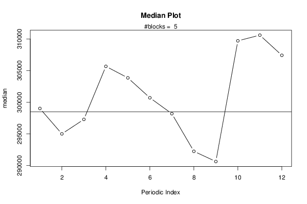
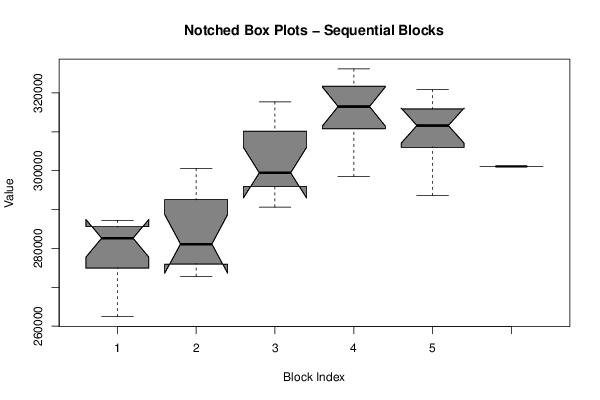
287224 279998 283495 285775 282329 277799 271980 266730 262433 285378 286692 282917 277686 274371 277466 290604 290770 283654 278601 274405 272817 294292 300562 298982 296917 295008 297295 305671 303853 300708 298194 292254 290646 314707 317009 317706 313312 311048 315917 326174 322116 317092 310468 302438 298493 320124 321873 321676 316696 312612 313307 320883 318749 315126 304600 295245 293619 309700 310597 307416 301126 | |||||||||||||||||||||
Tables (Output of Computation) | |||||||||||||||||||||
| |||||||||||||||||||||
Figures (Output of Computation) | |||||||||||||||||||||
Input Parameters & R Code | |||||||||||||||||||||
| Parameters (Session): | |||||||||||||||||||||
| par1 = 12 ; | |||||||||||||||||||||
| Parameters (R input): | |||||||||||||||||||||
| par1 = 12 ; | |||||||||||||||||||||
| R code (references can be found in the software module): | |||||||||||||||||||||
par1 <- as.numeric(par1) | |||||||||||||||||||||