Free Statistics
of Irreproducible Research!
Description of Statistical Computation | |||||||||||||||||||||||||
|---|---|---|---|---|---|---|---|---|---|---|---|---|---|---|---|---|---|---|---|---|---|---|---|---|---|
| Author's title | |||||||||||||||||||||||||
| Author | *The author of this computation has been verified* | ||||||||||||||||||||||||
| R Software Module | rwasp_Bayesian_Two_Sample_Test.wasp | ||||||||||||||||||||||||
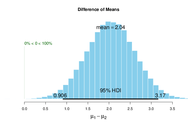
| Title produced by software | Bayesian Two Sample Test | ||||||||||||||||||||||||
| Date of computation | Sat, 28 Nov 2015 12:46:31 +0000 | ||||||||||||||||||||||||
| Cite this page as follows | Statistical Computations at FreeStatistics.org, Office for Research Development and Education, URL https://freestatistics.org/blog/index.php?v=date/2015/Nov/28/t1448714834mpfqcjnv02i3i6y.htm/, Retrieved Tue, 14 May 2024 22:59:56 +0000 | ||||||||||||||||||||||||
| Statistical Computations at FreeStatistics.org, Office for Research Development and Education, URL https://freestatistics.org/blog/index.php?pk=284376, Retrieved Tue, 14 May 2024 22:59:56 +0000 | |||||||||||||||||||||||||
| QR Codes: | |||||||||||||||||||||||||
|
| |||||||||||||||||||||||||
| Original text written by user: | |||||||||||||||||||||||||
| IsPrivate? | No (this computation is public) | ||||||||||||||||||||||||
| User-defined keywords | |||||||||||||||||||||||||
| Estimated Impact | 123 | ||||||||||||||||||||||||
Tree of Dependent Computations | |||||||||||||||||||||||||
| Family? (F = Feedback message, R = changed R code, M = changed R Module, P = changed Parameters, D = changed Data) | |||||||||||||||||||||||||
| - [Bayesian Two Sample Test] [Bayesian test wer...] [2015-11-28 12:46:31] [8acc4c3875a0c63009483cc7dfb4f316] [Current] - PD [Bayesian Two Sample Test] [Bayesian test wer...] [2015-12-01 13:54:44] [2ba32e9656c7c3fdddad3ba3f1588288] - RM [Multiple Regression] [Multiple regression] [2015-12-04 13:41:12] [4e6b221caf797a012ce5465db674848b] - RM D [] [Multiple regression] [-0001-11-30 00:00:00] [74be16979710d4c4e7c6647856088456] - RM D [] [Multiple regressi...] [-0001-11-30 00:00:00] [74be16979710d4c4e7c6647856088456] - RM [Multiple Regression] [Multiple regression] [2015-12-04 13:58:21] [4e6b221caf797a012ce5465db674848b] | |||||||||||||||||||||||||
| Feedback Forum | |||||||||||||||||||||||||
Post a new message | |||||||||||||||||||||||||
Dataset | |||||||||||||||||||||||||
| Dataseries X: | |||||||||||||||||||||||||
21.6 20.7 6.5 7.1 21.6 20.7 6.2 6.8 21.6 20.7 6.3 6.5 19.4 18 6.4 6.1 19.4 18 6.3 5.7 19.4 18 6.1 5.6 15.9 16.9 5.7 5.7 15.9 16.9 5.6 5.8 15.9 16.9 5.6 5.9 21.8 24.4 6.2 6.3 21.8 24.4 6.3 6.5 21.8 24.4 6.2 6.3 17.6 15.5 6 6.4 17.6 15.5 5.9 6.3 17.6 15.5 6 6.3 19 18.4 6.1 6.2 19 18.4 6.1 6.2 19 18.4 6 6.2 16.3 16.2 6 6.4 16.3 16.2 6 6.5 16.3 16.2 5.9 6.5 22.5 20.6 6.1 6.7 22.5 20.6 6.3 6.7 22.5 20.6 6.5 6.3 23.8 19.8 7.1 6.2 23.8 19.8 7.5 6.3 23.8 19.8 7.6 6.5 24.6 21.6 7.6 6.9 24.6 21.6 7.4 7 24.6 21.6 7.1 7 22.7 22.3 6.9 6.9 22.7 22.3 6.8 6.7 22.7 22.3 6.8 6.7 25.2 23.7 7.3 7.1 25.2 23.7 7.3 7.1 25.2 23.7 7.3 6.9 26.4 22.1 7.2 7 26.4 22.1 7.2 6.9 26.4 22.1 7.4 6.9 26 26.6 7.7 6.8 26 26.6 7.8 6.5 26 26.6 7.9 6.2 23.2 23.5 7.9 5.9 23.2 23.5 7.8 5.8 23.2 23.5 7.7 6.1 22.7 19.6 7.9 7 22.7 19.6 7.8 7.4 22.7 19.6 7.6 7.3 24 20 7.5 7.2 24 20 7.4 7.1 24 20 7.7 7.1 20.7 20.1 8.2 7.1 20.7 20.1 8.4 7.1 20.7 20.1 8.4 6.9 23.8 16 8.2 6.6 23.8 16 8 6.4 23.8 16 8 6.5 27.1 18.9 8.2 6.9 27.1 18.9 8.2 6.9 27.1 18.9 8 6.7 | |||||||||||||||||||||||||
Tables (Output of Computation) | |||||||||||||||||||||||||
| |||||||||||||||||||||||||
Figures (Output of Computation) | |||||||||||||||||||||||||
Input Parameters & R Code | |||||||||||||||||||||||||
| Parameters (Session): | |||||||||||||||||||||||||
| par1 = 1 ; par2 = 2 ; par3 = 0 ; par4 = 0.95 ; par5 = unpaired ; par6 = no ; | |||||||||||||||||||||||||
| Parameters (R input): | |||||||||||||||||||||||||
| par1 = 1 ; par2 = 2 ; par3 = 0 ; par4 = 0.95 ; par5 = unpaired ; par6 = no ; par7 = ; par8 = ; par9 = ; par10 = ; par11 = ; par12 = ; par13 = ; par14 = ; par15 = ; par16 = ; | |||||||||||||||||||||||||
| R code (references can be found in the software module): | |||||||||||||||||||||||||
library(BEST) | |||||||||||||||||||||||||