Free Statistics
of Irreproducible Research!
Description of Statistical Computation | |||||||||||||||||||||
|---|---|---|---|---|---|---|---|---|---|---|---|---|---|---|---|---|---|---|---|---|---|
| Author's title | |||||||||||||||||||||
| Author | *The author of this computation has been verified* | ||||||||||||||||||||
| R Software Module | rwasp_meanplot.wasp | ||||||||||||||||||||
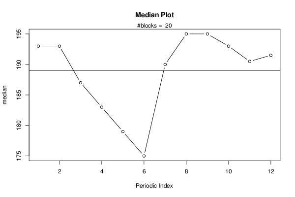
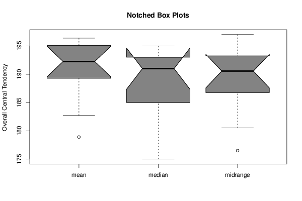
| Title produced by software | Mean Plot | ||||||||||||||||||||
| Date of computation | Thu, 26 Nov 2015 11:10:32 +0000 | ||||||||||||||||||||
| Cite this page as follows | Statistical Computations at FreeStatistics.org, Office for Research Development and Education, URL https://freestatistics.org/blog/index.php?v=date/2015/Nov/26/t1448536256tnjyrkfl4172yvf.htm/, Retrieved Tue, 14 May 2024 11:53:32 +0000 | ||||||||||||||||||||
| Statistical Computations at FreeStatistics.org, Office for Research Development and Education, URL https://freestatistics.org/blog/index.php?pk=284189, Retrieved Tue, 14 May 2024 11:53:32 +0000 | |||||||||||||||||||||
| QR Codes: | |||||||||||||||||||||
|
| |||||||||||||||||||||
| Original text written by user: | |||||||||||||||||||||
| IsPrivate? | No (this computation is public) | ||||||||||||||||||||
| User-defined keywords | |||||||||||||||||||||
| Estimated Impact | 129 | ||||||||||||||||||||
Tree of Dependent Computations | |||||||||||||||||||||
| Family? (F = Feedback message, R = changed R code, M = changed R Module, P = changed Parameters, D = changed Data) | |||||||||||||||||||||
| - [Central Tendency] [Arabica Price in ...] [2008-01-06 21:28:17] [74be16979710d4c4e7c6647856088456] - R D [Central Tendency] [Rekenkundig gemid...] [2015-11-25 11:25:04] [2e6b1bdc398efa0639617f5108875d85] - RMPD [Mean Plot] [Seizoenaliteit we...] [2015-11-26 11:10:32] [417cd1fa2ccbc3df120e1b65b71e6aee] [Current] | |||||||||||||||||||||
| Feedback Forum | |||||||||||||||||||||
Post a new message | |||||||||||||||||||||
Dataset | |||||||||||||||||||||
| Dataseries X: | |||||||||||||||||||||
191 189 184 179 175 171 179 191 195 195 193 193 195 193 187 181 176 169 174 185 186 182 178 178 179 178 174 171 168 167 175 187 191 188 185 185 187 188 186 183 179 176 183 198 203 198 192 191 194 194 192 188 182 175 178 181 171 164 159 160 163 159 148 139 129 124 136 146 143 141 135 134 135 134 136 142 142 135 140 146 155 170 167 166 160 156 156 160 156 150 157 158 167 189 197 199 193 188 186 190 186 181 190 189 192 201 200 206 208 202 190 171 163 167 195 208 208 197 189 192 199 202 200 191 190 180 194 196 199 200 199 205 207 211 210 208 201 186 177 168 173 181 185 186 189 186 181 182 176 165 176 174 168 165 162 170 179 178 169 160 151 159 191 195 184 162 152 162 188 202 209 204 193 191 202 204 206 211 214 224 224 222 219 218 213 213 229 225 220 212 204 204 202 195 186 175 170 171 196 202 200 191 186 186 193 193 188 185 182 180 194 204 216 233 241 243 241 233 228 225 219 217 235 237 238 235 234 239 248 248 247 246 240 233 242 239 238 238 238 240 249 251 253 251 246 247 260 260 259 | |||||||||||||||||||||
Tables (Output of Computation) | |||||||||||||||||||||
| |||||||||||||||||||||
Figures (Output of Computation) | |||||||||||||||||||||
Input Parameters & R Code | |||||||||||||||||||||
| Parameters (Session): | |||||||||||||||||||||
| par1 = 12 ; | |||||||||||||||||||||
| Parameters (R input): | |||||||||||||||||||||
| par1 = 12 ; | |||||||||||||||||||||
| R code (references can be found in the software module): | |||||||||||||||||||||
par1 <- as.numeric(par1) | |||||||||||||||||||||