Free Statistics
of Irreproducible Research!
Description of Statistical Computation | |||||||||||||||||||||
|---|---|---|---|---|---|---|---|---|---|---|---|---|---|---|---|---|---|---|---|---|---|
| Author's title | |||||||||||||||||||||
| Author | *The author of this computation has been verified* | ||||||||||||||||||||
| R Software Module | rwasp_meanplot.wasp | ||||||||||||||||||||
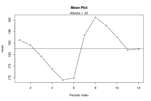
| Title produced by software | Mean Plot | ||||||||||||||||||||
| Date of computation | Thu, 26 Nov 2015 10:31:17 +0000 | ||||||||||||||||||||
| Cite this page as follows | Statistical Computations at FreeStatistics.org, Office for Research Development and Education, URL https://freestatistics.org/blog/index.php?v=date/2015/Nov/26/t1448536064gnuf05wpezvc4do.htm/, Retrieved Tue, 14 May 2024 09:47:31 +0000 | ||||||||||||||||||||
| Statistical Computations at FreeStatistics.org, Office for Research Development and Education, URL https://freestatistics.org/blog/index.php?pk=284188, Retrieved Tue, 14 May 2024 09:47:31 +0000 | |||||||||||||||||||||
| QR Codes: | |||||||||||||||||||||
|
| |||||||||||||||||||||
| Original text written by user: | |||||||||||||||||||||
| IsPrivate? | No (this computation is public) | ||||||||||||||||||||
| User-defined keywords | |||||||||||||||||||||
| Estimated Impact | 152 | ||||||||||||||||||||
Tree of Dependent Computations | |||||||||||||||||||||
| Family? (F = Feedback message, R = changed R code, M = changed R Module, P = changed Parameters, D = changed Data) | |||||||||||||||||||||
| - [Central Tendency] [Arabica Price in ...] [2008-01-06 21:28:17] [74be16979710d4c4e7c6647856088456] - R D [Central Tendency] [Rekenkundig gemid...] [2015-11-25 11:25:04] [2e6b1bdc398efa0639617f5108875d85] - RMPD [Mean Plot] [Seizonaliteit wer...] [2015-11-26 10:31:17] [417cd1fa2ccbc3df120e1b65b71e6aee] [Current] | |||||||||||||||||||||
| Feedback Forum | |||||||||||||||||||||
Post a new message | |||||||||||||||||||||
Dataset | |||||||||||||||||||||
| Dataseries X: | |||||||||||||||||||||
221 219 214 210 207 206 217 231 234 233 228 226 227 225 219 215 210 206 215 228 229 222 215 212 211 208 205 201 198 198 210 224 226 222 216 215 215 214 211 207 203 200 209 223 225 216 206 203 203 201 197 192 187 184 194 203 197 191 182 175 163 155 151 156 154 153 167 177 171 169 160 151 139 130 126 130 127 122 129 135 142 156 157 165 170 169 162 148 143 146 175 181 178 166 161 164 173 174 167 156 148 150 174 181 183 178 176 184 193 192 182 163 157 167 205 219 214 198 183 184 192 196 194 185 181 184 206 210 208 197 189 190 191 190 187 184 183 184 203 208 205 195 189 188 190 190 190 193 185 173 176 170 163 170 171 173 171 162 152 142 136 146 179 191 181 170 161 168 180 182 176 164 154 160 189 196 186 171 169 181 198 202 196 183 173 175 198 203 197 191 182 172 158 147 143 146 147 152 177 184 174 162 157 155 159 158 156 157 156 158 173 179 172 169 168 172 180 182 182 181 178 178 196 199 192 187 184 184 188 183 176 168 163 166 189 195 192 189 187 187 190 187 179 168 160 161 177 182 176 | |||||||||||||||||||||
Tables (Output of Computation) | |||||||||||||||||||||
| |||||||||||||||||||||
Figures (Output of Computation) | |||||||||||||||||||||
Input Parameters & R Code | |||||||||||||||||||||
| Parameters (Session): | |||||||||||||||||||||
| par1 = 12 ; | |||||||||||||||||||||
| Parameters (R input): | |||||||||||||||||||||
| par1 = 12 ; | |||||||||||||||||||||
| R code (references can be found in the software module): | |||||||||||||||||||||
par1 <- as.numeric(par1) | |||||||||||||||||||||