Repository of Reproducible Computations

Free Statistics

of Irreproducible Research!

Author's title

Author

*Unverified author*

R Software Module

rwasp_decompose.wasp

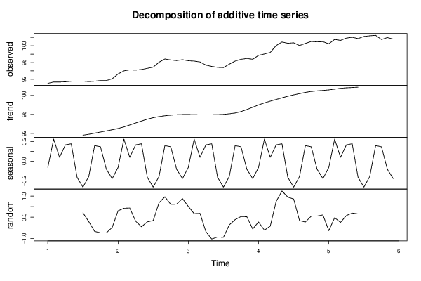
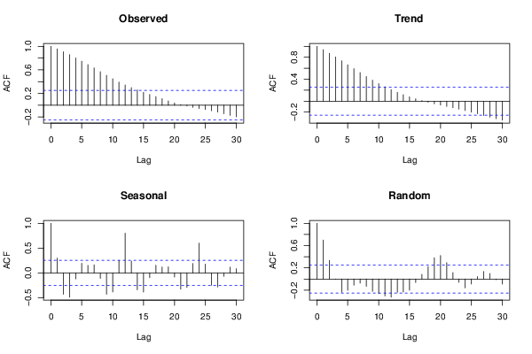
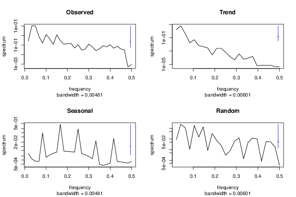
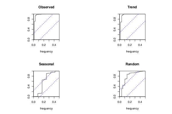
Title produced by software

Classical Decomposition

Date of computation

Mon, 23 Nov 2015 17:25:39 +0000

Cite this page as follows

Statistical Computations at FreeStatistics.org, Office for Research Development and Education, URL https://freestatistics.org/blog/index.php?v=date/2015/Nov/23/t1448299556l9kjeksyz3g3orn.htm/, Retrieved Tue, 14 May 2024 20:35:29 +0000

Statistical Computations at FreeStatistics.org, Office for Research Development and Education, URL https://freestatistics.org/blog/index.php?pk=283940, Retrieved Tue, 14 May 2024 20:35:29 +0000

QR Codes:

Paste this QR Code to cite your computation.

Original text written by user:

IsPrivate?

No (this computation is public)

User-defined keywords

Estimated Impact

106

Family? (F = Feedback message, R = changed R code, M = changed R Module, P = changed Parameters, D = changed Data)

-       [Classical Decomposition] [] [2015-11-23 17:25:39] [6fd7700de5d30cc4c677a9c8831c6222] [Current]

Feedback Forum

Post a new message

Dataseries X:

Download CSV

Histogram

Boxplots

Summary of computational transaction
Raw Input	view raw input (R code)
Raw Output	view raw output of R engine
Computing time	2 seconds
R Server	'Herman Ole Andreas Wold' @ wold.wessa.net

\begin{tabular}{lllllllll}
\hline
Summary of computational transaction \tabularnewline
Raw Input & view raw input (R code)  \tabularnewline
Raw Output & view raw output of R engine  \tabularnewline
Computing time & 2 seconds \tabularnewline
R Server & 'Herman Ole Andreas Wold' @ wold.wessa.net \tabularnewline
\hline
\end{tabular}
%Source: https://freestatistics.org/blog/index.php?pk=283940&T=0

[TABLE]
[ROW][C]Summary of computational transaction[/C][/ROW]
[ROW][C]Raw Input[/C][C]view raw input (R code) [/C][/ROW]
[ROW][C]Raw Output[/C][C]view raw output of R engine [/C][/ROW]
[ROW][C]Computing time[/C][C]2 seconds[/C][/ROW]
[ROW][C]R Server[/C][C]'Herman Ole Andreas Wold' @ wold.wessa.net[/C][/ROW]
[/TABLE]
Source: https://freestatistics.org/blog/index.php?pk=283940&T=0

Globally Unique Identifier (entire table): ba.freestatistics.org/blog/index.php?pk=283940&T=0

As an alternative you can also use a QR Code:

The GUIDs for individual cells are displayed in the table below:

Summary of computational transaction
Raw Input	view raw input (R code)
Raw Output	view raw output of R engine
Computing time	2 seconds
R Server	'Herman Ole Andreas Wold' @ wold.wessa.net

Classical Decomposition by Moving Averages
t	Observations	Fit	Trend	Seasonal	Random
1	91.04	NA	NA	-0.0640365	NA
2	91.37	NA	NA	0.223776	NA
3	91.36	NA	NA	0.0385677	NA
4	91.4	NA	NA	0.165026	NA
5	91.54	NA	NA	0.176276	NA
6	91.57	NA	NA	-0.164349	NA
7	91.57	91.3635	91.6275	-0.264036	0.206536
8	91.47	91.6759	91.8312	-0.155391	-0.205859
9	91.55	92.2204	92.0625	0.157943	-0.670443
10	91.71	92.4453	92.2996	0.145755	-0.735339
11	91.71	92.4502	92.5325	-0.0822656	-0.740234
12	92.12	92.599	92.7762	-0.177266	-0.478984
13	93.28	92.978	93.0421	-0.0640365	0.301953
14	94.02	93.5967	93.3729	0.223776	0.423307
15	94.26	93.8244	93.7858	0.0385677	0.435599
16	94.19	94.3759	94.2108	0.165026	-0.185859
17	94.34	94.7896	94.6133	0.176276	-0.449609
18	94.62	94.8373	95.0017	-0.164349	-0.217318
19	94.9	95.0589	95.3229	-0.264036	-0.15888
20	96.08	95.3959	95.5512	-0.155391	0.684141
21	96.85	95.8846	95.7267	0.157943	0.965391
22	96.61	96.0008	95.855	0.145755	0.609245
23	96.47	95.8536	95.9358	-0.0822656	0.616432
24	96.68	95.7994	95.9767	-0.177266	0.880599
25	96.43	95.9185	95.9825	-0.0640365	0.511536
26	96.35	96.1829	95.9592	0.223776	0.167057
27	96.14	95.9577	95.9192	0.0385677	0.182266
28	95.39	96.07	95.905	0.165026	-0.680026
29	95.08	96.1088	95.9325	0.176276	-1.02878
30	94.86	95.7932	95.9575	-0.164349	-0.933151
31	94.8	95.751	96.015	-0.264036	-0.950964
32	95.62	95.9834	96.1387	-0.155391	-0.363359
33	96.35	96.4617	96.3037	0.157943	-0.111693
34	96.77	96.7383	96.5925	0.145755	0.0317448
35	96.97	96.9469	97.0292	-0.0822656	0.023099
36	96.78	97.334	97.5112	-0.177266	-0.553984
37	97.71	97.933	97.9971	-0.0640365	-0.223047
38	98.04	98.6521	98.4283	0.223776	-0.612109
39	98.41	98.8277	98.7892	0.0385677	-0.417734
40	100.05	99.3075	99.1425	0.165026	0.742474
41	100.9	99.6613	99.485	0.176276	1.23872
42	100.61	99.6607	99.825	-0.164349	0.949349
43	100.71	99.8505	100.115	-0.264036	0.859453
44	100.06	100.219	100.374	-0.155391	-0.158776
45	100.57	100.797	100.639	0.157943	-0.227109
46	101.03	100.98	100.834	0.145755	0.0504948
47	100.93	100.873	100.955	-0.0822656	0.056849
48	100.98	100.871	101.049	-0.177266	0.108516
49	100.46	101.094	101.158	-0.0640365	-0.634297
50	101.52	101.542	101.318	0.223776	-0.0221094
51	101.29	101.534	101.495	0.0385677	-0.243984
52	101.84	101.76	101.595	0.165026	0.0795573
53	102.03	101.834	101.658	0.176276	0.195807
54	101.72	101.563	101.727	-0.164349	0.157266
55	102.23	NA	NA	-0.264036	NA
56	102.38	NA	NA	-0.155391	NA
57	102.5	NA	NA	0.157943	NA
58	101.5	NA	NA	0.145755	NA
59	101.96	NA	NA	-0.0822656	NA
60	101.61	NA	NA	-0.177266	NA

\begin{tabular}{lllllllll}
\hline
Classical Decomposition by Moving Averages \tabularnewline
t & Observations & Fit & Trend & Seasonal & Random \tabularnewline
1 & 91.04 & NA & NA & -0.0640365 & NA \tabularnewline
2 & 91.37 & NA & NA & 0.223776 & NA \tabularnewline
3 & 91.36 & NA & NA & 0.0385677 & NA \tabularnewline
4 & 91.4 & NA & NA & 0.165026 & NA \tabularnewline
5 & 91.54 & NA & NA & 0.176276 & NA \tabularnewline
6 & 91.57 & NA & NA & -0.164349 & NA \tabularnewline
7 & 91.57 & 91.3635 & 91.6275 & -0.264036 & 0.206536 \tabularnewline
8 & 91.47 & 91.6759 & 91.8312 & -0.155391 & -0.205859 \tabularnewline
9 & 91.55 & 92.2204 & 92.0625 & 0.157943 & -0.670443 \tabularnewline
10 & 91.71 & 92.4453 & 92.2996 & 0.145755 & -0.735339 \tabularnewline
11 & 91.71 & 92.4502 & 92.5325 & -0.0822656 & -0.740234 \tabularnewline
12 & 92.12 & 92.599 & 92.7762 & -0.177266 & -0.478984 \tabularnewline
13 & 93.28 & 92.978 & 93.0421 & -0.0640365 & 0.301953 \tabularnewline
14 & 94.02 & 93.5967 & 93.3729 & 0.223776 & 0.423307 \tabularnewline
15 & 94.26 & 93.8244 & 93.7858 & 0.0385677 & 0.435599 \tabularnewline
16 & 94.19 & 94.3759 & 94.2108 & 0.165026 & -0.185859 \tabularnewline
17 & 94.34 & 94.7896 & 94.6133 & 0.176276 & -0.449609 \tabularnewline
18 & 94.62 & 94.8373 & 95.0017 & -0.164349 & -0.217318 \tabularnewline
19 & 94.9 & 95.0589 & 95.3229 & -0.264036 & -0.15888 \tabularnewline
20 & 96.08 & 95.3959 & 95.5512 & -0.155391 & 0.684141 \tabularnewline
21 & 96.85 & 95.8846 & 95.7267 & 0.157943 & 0.965391 \tabularnewline
22 & 96.61 & 96.0008 & 95.855 & 0.145755 & 0.609245 \tabularnewline
23 & 96.47 & 95.8536 & 95.9358 & -0.0822656 & 0.616432 \tabularnewline
24 & 96.68 & 95.7994 & 95.9767 & -0.177266 & 0.880599 \tabularnewline
25 & 96.43 & 95.9185 & 95.9825 & -0.0640365 & 0.511536 \tabularnewline
26 & 96.35 & 96.1829 & 95.9592 & 0.223776 & 0.167057 \tabularnewline
27 & 96.14 & 95.9577 & 95.9192 & 0.0385677 & 0.182266 \tabularnewline
28 & 95.39 & 96.07 & 95.905 & 0.165026 & -0.680026 \tabularnewline
29 & 95.08 & 96.1088 & 95.9325 & 0.176276 & -1.02878 \tabularnewline
30 & 94.86 & 95.7932 & 95.9575 & -0.164349 & -0.933151 \tabularnewline
31 & 94.8 & 95.751 & 96.015 & -0.264036 & -0.950964 \tabularnewline
32 & 95.62 & 95.9834 & 96.1387 & -0.155391 & -0.363359 \tabularnewline
33 & 96.35 & 96.4617 & 96.3037 & 0.157943 & -0.111693 \tabularnewline
34 & 96.77 & 96.7383 & 96.5925 & 0.145755 & 0.0317448 \tabularnewline
35 & 96.97 & 96.9469 & 97.0292 & -0.0822656 & 0.023099 \tabularnewline
36 & 96.78 & 97.334 & 97.5112 & -0.177266 & -0.553984 \tabularnewline
37 & 97.71 & 97.933 & 97.9971 & -0.0640365 & -0.223047 \tabularnewline
38 & 98.04 & 98.6521 & 98.4283 & 0.223776 & -0.612109 \tabularnewline
39 & 98.41 & 98.8277 & 98.7892 & 0.0385677 & -0.417734 \tabularnewline
40 & 100.05 & 99.3075 & 99.1425 & 0.165026 & 0.742474 \tabularnewline
41 & 100.9 & 99.6613 & 99.485 & 0.176276 & 1.23872 \tabularnewline
42 & 100.61 & 99.6607 & 99.825 & -0.164349 & 0.949349 \tabularnewline
43 & 100.71 & 99.8505 & 100.115 & -0.264036 & 0.859453 \tabularnewline
44 & 100.06 & 100.219 & 100.374 & -0.155391 & -0.158776 \tabularnewline
45 & 100.57 & 100.797 & 100.639 & 0.157943 & -0.227109 \tabularnewline
46 & 101.03 & 100.98 & 100.834 & 0.145755 & 0.0504948 \tabularnewline
47 & 100.93 & 100.873 & 100.955 & -0.0822656 & 0.056849 \tabularnewline
48 & 100.98 & 100.871 & 101.049 & -0.177266 & 0.108516 \tabularnewline
49 & 100.46 & 101.094 & 101.158 & -0.0640365 & -0.634297 \tabularnewline
50 & 101.52 & 101.542 & 101.318 & 0.223776 & -0.0221094 \tabularnewline
51 & 101.29 & 101.534 & 101.495 & 0.0385677 & -0.243984 \tabularnewline
52 & 101.84 & 101.76 & 101.595 & 0.165026 & 0.0795573 \tabularnewline
53 & 102.03 & 101.834 & 101.658 & 0.176276 & 0.195807 \tabularnewline
54 & 101.72 & 101.563 & 101.727 & -0.164349 & 0.157266 \tabularnewline
55 & 102.23 & NA & NA & -0.264036 & NA \tabularnewline
56 & 102.38 & NA & NA & -0.155391 & NA \tabularnewline
57 & 102.5 & NA & NA & 0.157943 & NA \tabularnewline
58 & 101.5 & NA & NA & 0.145755 & NA \tabularnewline
59 & 101.96 & NA & NA & -0.0822656 & NA \tabularnewline
60 & 101.61 & NA & NA & -0.177266 & NA \tabularnewline
\hline
\end{tabular}
%Source: https://freestatistics.org/blog/index.php?pk=283940&T=1

[TABLE]
[ROW][C]Classical Decomposition by Moving Averages[/C][/ROW]
[ROW][C]t[/C][C]Observations[/C][C]Fit[/C][C]Trend[/C][C]Seasonal[/C][C]Random[/C][/ROW]
[ROW][C]1[/C][C]91.04[/C][C]NA[/C][C]NA[/C][C]-0.0640365[/C][C]NA[/C][/ROW]
[ROW][C]2[/C][C]91.37[/C][C]NA[/C][C]NA[/C][C]0.223776[/C][C]NA[/C][/ROW]
[ROW][C]3[/C][C]91.36[/C][C]NA[/C][C]NA[/C][C]0.0385677[/C][C]NA[/C][/ROW]
[ROW][C]4[/C][C]91.4[/C][C]NA[/C][C]NA[/C][C]0.165026[/C][C]NA[/C][/ROW]
[ROW][C]5[/C][C]91.54[/C][C]NA[/C][C]NA[/C][C]0.176276[/C][C]NA[/C][/ROW]
[ROW][C]6[/C][C]91.57[/C][C]NA[/C][C]NA[/C][C]-0.164349[/C][C]NA[/C][/ROW]
[ROW][C]7[/C][C]91.57[/C][C]91.3635[/C][C]91.6275[/C][C]-0.264036[/C][C]0.206536[/C][/ROW]
[ROW][C]8[/C][C]91.47[/C][C]91.6759[/C][C]91.8312[/C][C]-0.155391[/C][C]-0.205859[/C][/ROW]
[ROW][C]9[/C][C]91.55[/C][C]92.2204[/C][C]92.0625[/C][C]0.157943[/C][C]-0.670443[/C][/ROW]
[ROW][C]10[/C][C]91.71[/C][C]92.4453[/C][C]92.2996[/C][C]0.145755[/C][C]-0.735339[/C][/ROW]
[ROW][C]11[/C][C]91.71[/C][C]92.4502[/C][C]92.5325[/C][C]-0.0822656[/C][C]-0.740234[/C][/ROW]
[ROW][C]12[/C][C]92.12[/C][C]92.599[/C][C]92.7762[/C][C]-0.177266[/C][C]-0.478984[/C][/ROW]
[ROW][C]13[/C][C]93.28[/C][C]92.978[/C][C]93.0421[/C][C]-0.0640365[/C][C]0.301953[/C][/ROW]
[ROW][C]14[/C][C]94.02[/C][C]93.5967[/C][C]93.3729[/C][C]0.223776[/C][C]0.423307[/C][/ROW]
[ROW][C]15[/C][C]94.26[/C][C]93.8244[/C][C]93.7858[/C][C]0.0385677[/C][C]0.435599[/C][/ROW]
[ROW][C]16[/C][C]94.19[/C][C]94.3759[/C][C]94.2108[/C][C]0.165026[/C][C]-0.185859[/C][/ROW]
[ROW][C]17[/C][C]94.34[/C][C]94.7896[/C][C]94.6133[/C][C]0.176276[/C][C]-0.449609[/C][/ROW]
[ROW][C]18[/C][C]94.62[/C][C]94.8373[/C][C]95.0017[/C][C]-0.164349[/C][C]-0.217318[/C][/ROW]
[ROW][C]19[/C][C]94.9[/C][C]95.0589[/C][C]95.3229[/C][C]-0.264036[/C][C]-0.15888[/C][/ROW]
[ROW][C]20[/C][C]96.08[/C][C]95.3959[/C][C]95.5512[/C][C]-0.155391[/C][C]0.684141[/C][/ROW]
[ROW][C]21[/C][C]96.85[/C][C]95.8846[/C][C]95.7267[/C][C]0.157943[/C][C]0.965391[/C][/ROW]
[ROW][C]22[/C][C]96.61[/C][C]96.0008[/C][C]95.855[/C][C]0.145755[/C][C]0.609245[/C][/ROW]
[ROW][C]23[/C][C]96.47[/C][C]95.8536[/C][C]95.9358[/C][C]-0.0822656[/C][C]0.616432[/C][/ROW]
[ROW][C]24[/C][C]96.68[/C][C]95.7994[/C][C]95.9767[/C][C]-0.177266[/C][C]0.880599[/C][/ROW]
[ROW][C]25[/C][C]96.43[/C][C]95.9185[/C][C]95.9825[/C][C]-0.0640365[/C][C]0.511536[/C][/ROW]
[ROW][C]26[/C][C]96.35[/C][C]96.1829[/C][C]95.9592[/C][C]0.223776[/C][C]0.167057[/C][/ROW]
[ROW][C]27[/C][C]96.14[/C][C]95.9577[/C][C]95.9192[/C][C]0.0385677[/C][C]0.182266[/C][/ROW]
[ROW][C]28[/C][C]95.39[/C][C]96.07[/C][C]95.905[/C][C]0.165026[/C][C]-0.680026[/C][/ROW]
[ROW][C]29[/C][C]95.08[/C][C]96.1088[/C][C]95.9325[/C][C]0.176276[/C][C]-1.02878[/C][/ROW]
[ROW][C]30[/C][C]94.86[/C][C]95.7932[/C][C]95.9575[/C][C]-0.164349[/C][C]-0.933151[/C][/ROW]
[ROW][C]31[/C][C]94.8[/C][C]95.751[/C][C]96.015[/C][C]-0.264036[/C][C]-0.950964[/C][/ROW]
[ROW][C]32[/C][C]95.62[/C][C]95.9834[/C][C]96.1387[/C][C]-0.155391[/C][C]-0.363359[/C][/ROW]
[ROW][C]33[/C][C]96.35[/C][C]96.4617[/C][C]96.3037[/C][C]0.157943[/C][C]-0.111693[/C][/ROW]
[ROW][C]34[/C][C]96.77[/C][C]96.7383[/C][C]96.5925[/C][C]0.145755[/C][C]0.0317448[/C][/ROW]
[ROW][C]35[/C][C]96.97[/C][C]96.9469[/C][C]97.0292[/C][C]-0.0822656[/C][C]0.023099[/C][/ROW]
[ROW][C]36[/C][C]96.78[/C][C]97.334[/C][C]97.5112[/C][C]-0.177266[/C][C]-0.553984[/C][/ROW]
[ROW][C]37[/C][C]97.71[/C][C]97.933[/C][C]97.9971[/C][C]-0.0640365[/C][C]-0.223047[/C][/ROW]
[ROW][C]38[/C][C]98.04[/C][C]98.6521[/C][C]98.4283[/C][C]0.223776[/C][C]-0.612109[/C][/ROW]
[ROW][C]39[/C][C]98.41[/C][C]98.8277[/C][C]98.7892[/C][C]0.0385677[/C][C]-0.417734[/C][/ROW]
[ROW][C]40[/C][C]100.05[/C][C]99.3075[/C][C]99.1425[/C][C]0.165026[/C][C]0.742474[/C][/ROW]
[ROW][C]41[/C][C]100.9[/C][C]99.6613[/C][C]99.485[/C][C]0.176276[/C][C]1.23872[/C][/ROW]
[ROW][C]42[/C][C]100.61[/C][C]99.6607[/C][C]99.825[/C][C]-0.164349[/C][C]0.949349[/C][/ROW]
[ROW][C]43[/C][C]100.71[/C][C]99.8505[/C][C]100.115[/C][C]-0.264036[/C][C]0.859453[/C][/ROW]
[ROW][C]44[/C][C]100.06[/C][C]100.219[/C][C]100.374[/C][C]-0.155391[/C][C]-0.158776[/C][/ROW]
[ROW][C]45[/C][C]100.57[/C][C]100.797[/C][C]100.639[/C][C]0.157943[/C][C]-0.227109[/C][/ROW]
[ROW][C]46[/C][C]101.03[/C][C]100.98[/C][C]100.834[/C][C]0.145755[/C][C]0.0504948[/C][/ROW]
[ROW][C]47[/C][C]100.93[/C][C]100.873[/C][C]100.955[/C][C]-0.0822656[/C][C]0.056849[/C][/ROW]
[ROW][C]48[/C][C]100.98[/C][C]100.871[/C][C]101.049[/C][C]-0.177266[/C][C]0.108516[/C][/ROW]
[ROW][C]49[/C][C]100.46[/C][C]101.094[/C][C]101.158[/C][C]-0.0640365[/C][C]-0.634297[/C][/ROW]
[ROW][C]50[/C][C]101.52[/C][C]101.542[/C][C]101.318[/C][C]0.223776[/C][C]-0.0221094[/C][/ROW]
[ROW][C]51[/C][C]101.29[/C][C]101.534[/C][C]101.495[/C][C]0.0385677[/C][C]-0.243984[/C][/ROW]
[ROW][C]52[/C][C]101.84[/C][C]101.76[/C][C]101.595[/C][C]0.165026[/C][C]0.0795573[/C][/ROW]
[ROW][C]53[/C][C]102.03[/C][C]101.834[/C][C]101.658[/C][C]0.176276[/C][C]0.195807[/C][/ROW]
[ROW][C]54[/C][C]101.72[/C][C]101.563[/C][C]101.727[/C][C]-0.164349[/C][C]0.157266[/C][/ROW]
[ROW][C]55[/C][C]102.23[/C][C]NA[/C][C]NA[/C][C]-0.264036[/C][C]NA[/C][/ROW]
[ROW][C]56[/C][C]102.38[/C][C]NA[/C][C]NA[/C][C]-0.155391[/C][C]NA[/C][/ROW]
[ROW][C]57[/C][C]102.5[/C][C]NA[/C][C]NA[/C][C]0.157943[/C][C]NA[/C][/ROW]
[ROW][C]58[/C][C]101.5[/C][C]NA[/C][C]NA[/C][C]0.145755[/C][C]NA[/C][/ROW]
[ROW][C]59[/C][C]101.96[/C][C]NA[/C][C]NA[/C][C]-0.0822656[/C][C]NA[/C][/ROW]
[ROW][C]60[/C][C]101.61[/C][C]NA[/C][C]NA[/C][C]-0.177266[/C][C]NA[/C][/ROW]
[/TABLE]
Source: https://freestatistics.org/blog/index.php?pk=283940&T=1

Globally Unique Identifier (entire table): ba.freestatistics.org/blog/index.php?pk=283940&T=1

As an alternative you can also use a QR Code:

The GUIDs for individual cells are displayed in the table below:

Classical Decomposition by Moving Averages
t	Observations	Fit	Trend	Seasonal	Random
1	91.04	NA	NA	-0.0640365	NA
2	91.37	NA	NA	0.223776	NA
3	91.36	NA	NA	0.0385677	NA
4	91.4	NA	NA	0.165026	NA
5	91.54	NA	NA	0.176276	NA
6	91.57	NA	NA	-0.164349	NA
7	91.57	91.3635	91.6275	-0.264036	0.206536
8	91.47	91.6759	91.8312	-0.155391	-0.205859
9	91.55	92.2204	92.0625	0.157943	-0.670443
10	91.71	92.4453	92.2996	0.145755	-0.735339
11	91.71	92.4502	92.5325	-0.0822656	-0.740234
12	92.12	92.599	92.7762	-0.177266	-0.478984
13	93.28	92.978	93.0421	-0.0640365	0.301953
14	94.02	93.5967	93.3729	0.223776	0.423307
15	94.26	93.8244	93.7858	0.0385677	0.435599
16	94.19	94.3759	94.2108	0.165026	-0.185859
17	94.34	94.7896	94.6133	0.176276	-0.449609
18	94.62	94.8373	95.0017	-0.164349	-0.217318
19	94.9	95.0589	95.3229	-0.264036	-0.15888
20	96.08	95.3959	95.5512	-0.155391	0.684141
21	96.85	95.8846	95.7267	0.157943	0.965391
22	96.61	96.0008	95.855	0.145755	0.609245
23	96.47	95.8536	95.9358	-0.0822656	0.616432
24	96.68	95.7994	95.9767	-0.177266	0.880599
25	96.43	95.9185	95.9825	-0.0640365	0.511536
26	96.35	96.1829	95.9592	0.223776	0.167057
27	96.14	95.9577	95.9192	0.0385677	0.182266
28	95.39	96.07	95.905	0.165026	-0.680026
29	95.08	96.1088	95.9325	0.176276	-1.02878
30	94.86	95.7932	95.9575	-0.164349	-0.933151
31	94.8	95.751	96.015	-0.264036	-0.950964
32	95.62	95.9834	96.1387	-0.155391	-0.363359
33	96.35	96.4617	96.3037	0.157943	-0.111693
34	96.77	96.7383	96.5925	0.145755	0.0317448
35	96.97	96.9469	97.0292	-0.0822656	0.023099
36	96.78	97.334	97.5112	-0.177266	-0.553984
37	97.71	97.933	97.9971	-0.0640365	-0.223047
38	98.04	98.6521	98.4283	0.223776	-0.612109
39	98.41	98.8277	98.7892	0.0385677	-0.417734
40	100.05	99.3075	99.1425	0.165026	0.742474
41	100.9	99.6613	99.485	0.176276	1.23872
42	100.61	99.6607	99.825	-0.164349	0.949349
43	100.71	99.8505	100.115	-0.264036	0.859453
44	100.06	100.219	100.374	-0.155391	-0.158776
45	100.57	100.797	100.639	0.157943	-0.227109
46	101.03	100.98	100.834	0.145755	0.0504948
47	100.93	100.873	100.955	-0.0822656	0.056849
48	100.98	100.871	101.049	-0.177266	0.108516
49	100.46	101.094	101.158	-0.0640365	-0.634297
50	101.52	101.542	101.318	0.223776	-0.0221094
51	101.29	101.534	101.495	0.0385677	-0.243984
52	101.84	101.76	101.595	0.165026	0.0795573
53	102.03	101.834	101.658	0.176276	0.195807
54	101.72	101.563	101.727	-0.164349	0.157266
55	102.23	NA	NA	-0.264036	NA
56	102.38	NA	NA	-0.155391	NA
57	102.5	NA	NA	0.157943	NA
58	101.5	NA	NA	0.145755	NA
59	101.96	NA	NA	-0.0822656	NA
60	101.61	NA	NA	-0.177266	NA

Figure 1

PNG link

Postscript link

PDF link

Figure 2

PNG link

Postscript link

PDF link

Figure 3

PNG link

Postscript link

PDF link

Figure 4

PNG link

Postscript link

PDF link

Parameters (Session):

par1 = additive ; par2 = 12 ;

Parameters (R input):

par1 = additive ; par2 = 12 ;

R code (references can be found in the software module):

par2 <- as.numeric(par2)
x <- ts(x,freq=par2)
m <- decompose(x,type=par1)
m$figure
bitmap(file='test1.png')
plot(m)
dev.off()
mylagmax <- length(x)/2
bitmap(file='test2.png')
op <- par(mfrow = c(2,2))
acf(as.numeric(x),lag.max = mylagmax,main='Observed')
acf(as.numeric(m$trend),na.action=na.pass,lag.max = mylagmax,main='Trend')
acf(as.numeric(m$seasonal),na.action=na.pass,lag.max = mylagmax,main='Seasonal')
acf(as.numeric(m$random),na.action=na.pass,lag.max = mylagmax,main='Random')
par(op)
dev.off()
bitmap(file='test3.png')
op <- par(mfrow = c(2,2))
spectrum(as.numeric(x),main='Observed')
spectrum(as.numeric(m$trend[!is.na(m$trend)]),main='Trend')
spectrum(as.numeric(m$seasonal[!is.na(m$seasonal)]),main='Seasonal')
spectrum(as.numeric(m$random[!is.na(m$random)]),main='Random')
par(op)
dev.off()
bitmap(file='test4.png')
op <- par(mfrow = c(2,2))
cpgram(as.numeric(x),main='Observed')
cpgram(as.numeric(m$trend[!is.na(m$trend)]),main='Trend')
cpgram(as.numeric(m$seasonal[!is.na(m$seasonal)]),main='Seasonal')
cpgram(as.numeric(m$random[!is.na(m$random)]),main='Random')
par(op)
dev.off()
load(file='createtable')
a<-table.start()
a<-table.row.start(a)
a<-table.element(a,'Classical Decomposition by Moving Averages',6,TRUE)
a<-table.row.end(a)
a<-table.row.start(a)
a<-table.element(a,'t',header=TRUE)
a<-table.element(a,'Observations',header=TRUE)
a<-table.element(a,'Fit',header=TRUE)
a<-table.element(a,'Trend',header=TRUE)
a<-table.element(a,'Seasonal',header=TRUE)
a<-table.element(a,'Random',header=TRUE)
a<-table.row.end(a)
for (i in 1:length(m$trend)) {
a<-table.row.start(a)
a<-table.element(a,i,header=TRUE)
a<-table.element(a,x[i])
if (par1 == 'additive') a<-table.element(a,signif(m$trend[i]+m$seasonal[i],6)) else a<-table.element(a,signif(m$trend[i]*m$seasonal[i],6))
a<-table.element(a,signif(m$trend[i],6))
a<-table.element(a,signif(m$seasonal[i],6))
a<-table.element(a,signif(m$random[i],6))
a<-table.row.end(a)
}
a<-table.end(a)
table.save(a,file='mytable.tab')

Free Statistics

Description of Statistical Computation

Tree of Dependent Computations

Dataset

Tables (Output of Computation)

Figures (Output of Computation)

Input Parameters & R Code