Free Statistics
of Irreproducible Research!
Description of Statistical Computation | |||||||||||||||||||||
|---|---|---|---|---|---|---|---|---|---|---|---|---|---|---|---|---|---|---|---|---|---|
| Author's title | |||||||||||||||||||||
| Author | *Unverified author* | ||||||||||||||||||||
| R Software Module | rwasp_sdplot.wasp | ||||||||||||||||||||
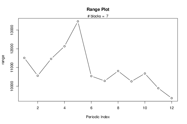
| Title produced by software | Standard Deviation Plot | ||||||||||||||||||||
| Date of computation | Sun, 22 Nov 2015 11:55:15 +0000 | ||||||||||||||||||||
| Cite this page as follows | Statistical Computations at FreeStatistics.org, Office for Research Development and Education, URL https://freestatistics.org/blog/index.php?v=date/2015/Nov/22/t1448193335y6cuty2hqd2l0dj.htm/, Retrieved Wed, 15 May 2024 05:30:14 +0000 | ||||||||||||||||||||
| Statistical Computations at FreeStatistics.org, Office for Research Development and Education, URL https://freestatistics.org/blog/index.php?pk=283784, Retrieved Wed, 15 May 2024 05:30:14 +0000 | |||||||||||||||||||||
| QR Codes: | |||||||||||||||||||||
|
| |||||||||||||||||||||
| Original text written by user: | |||||||||||||||||||||
| IsPrivate? | No (this computation is public) | ||||||||||||||||||||
| User-defined keywords | |||||||||||||||||||||
| Estimated Impact | 133 | ||||||||||||||||||||
Tree of Dependent Computations | |||||||||||||||||||||
| Family? (F = Feedback message, R = changed R code, M = changed R Module, P = changed Parameters, D = changed Data) | |||||||||||||||||||||
| - [Variability] [] [2015-11-22 11:43:11] [553dab97a9d8b6d0026004b85d73532b] - RMPD [Standard Deviation Plot] [] [2015-11-22 11:55:15] [a9d02bc5e77e4ed95e8bc9cdb21bd9af] [Current] | |||||||||||||||||||||
| Feedback Forum | |||||||||||||||||||||
Post a new message | |||||||||||||||||||||
Dataset | |||||||||||||||||||||
| Dataseries X: | |||||||||||||||||||||
31025 31068 31619 32020 30467 31960 31389 28863 33143 33350 29079 26505 24975 24644 26626 23977 23898 25583 25974 23529 27491 28053 27913 26706 26788 27600 32770 29623 29300 32152 30700 29463 32709 32823 34073 33551 32168 32833 37341 33747 34482 33309 33057 32809 35316 33989 35799 34508 34646 35203 38084 35005 36734 35716 34543 34340 35094 38730 37805 33815 36486 34960 38054 35283 37361 35536 36103 33886 35416 38053 37181 34787 36074 34966 37482 36109 35520 36123 36256 32456 37748 38461 36344 35865 | |||||||||||||||||||||
Tables (Output of Computation) | |||||||||||||||||||||
| |||||||||||||||||||||
Figures (Output of Computation) | |||||||||||||||||||||
Input Parameters & R Code | |||||||||||||||||||||
| Parameters (Session): | |||||||||||||||||||||
| par1 = 12 ; | |||||||||||||||||||||
| Parameters (R input): | |||||||||||||||||||||
| par1 = 12 ; | |||||||||||||||||||||
| R code (references can be found in the software module): | |||||||||||||||||||||
par1 <- as.numeric(par1) | |||||||||||||||||||||