Repository of Reproducible Computations

Free Statistics

of Irreproducible Research!

Author's title

Author

*The author of this computation has been verified*

R Software Module

rwasp_fitdistrnorm.wasp

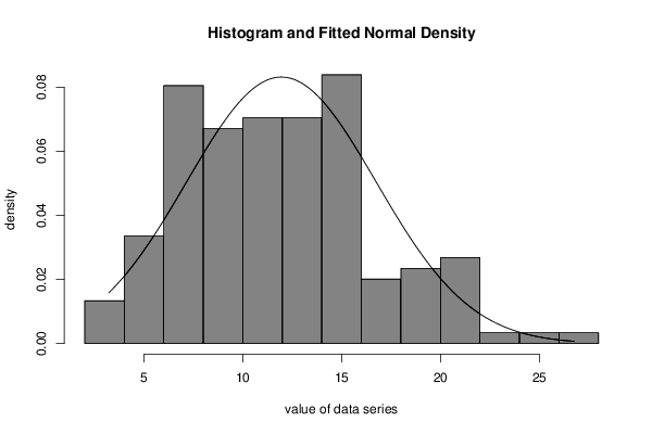
Title produced by software

ML Fitting and QQ Plot- Normal Distribution

Date of computation

Sat, 21 Nov 2015 11:12:11 +0000

Cite this page as follows

Statistical Computations at FreeStatistics.org, Office for Research Development and Education, URL https://freestatistics.org/blog/index.php?v=date/2015/Nov/21/t1448104475bwlpgz4n5fqwg8f.htm/, Retrieved Tue, 14 May 2024 08:40:02 +0000

Statistical Computations at FreeStatistics.org, Office for Research Development and Education, URL https://freestatistics.org/blog/index.php?pk=283749, Retrieved Tue, 14 May 2024 08:40:02 +0000

QR Codes:

Paste this QR Code to cite your computation.

Original text written by user:

we zien opnieuw geen normaalverdeling in het histogram

IsPrivate?

No (this computation is public)

User-defined keywords

Estimated Impact

118

Family? (F = Feedback message, R = changed R code, M = changed R Module, P = changed Parameters, D = changed Data)

-       [ML Fitting and QQ Plot- Normal Distribution] [3.1 task 4 ] [2015-11-21 11:12:11] [bfb327cc38fccc6d3daed2ac8fd9ce3b] [Current]

Feedback Forum

Post a new message

Dataseries X:

Download CSV

Histogram

Boxplots

11.28213147
19.80976738
14.68725698
18.24650513
13.41384973
11.06389324
9.448028228
6.626878796
12.67032425
13.85249866
5.827720375
13.42563838
13.87352764
7.702996539
21.45831683
11.41456151
14.90524342
15.69843882
9.940968653
13.47435426
10.09514188
26.77186892
3.616551467
8.787921821
14.43049419
14.34610876
17.27412249
7.838995367
19.23249398
13.99180483
6.07853677
13.77494623
8.552342548
9.222865946
20.96687335
18.92515854
6.751124117
13.99710458
13.668061
12.29080775
7.49616521
14.20439884
12.42500634
11.34422843
9.805490973
17.65550643
24.14277747
8.223136808
10.8113172
8.889826106
6.938388402
17.59084112
10.14508619
15.25291132
7.845452531
15.61462373
7.299101692
9.780458111
10.98151097
15.38552714
15.90571297
6.389202182
12.27389423
20.70376358
12.64326228
11.06932013
6.018691925
20.49527356
11.09215162
14.99159978
20.08656489
10.77515701
6.856662284
9.460471204
20.15421393
16.26630398
20.33885739
9.04785309
10.60225122
11.08780214
11.90266828
3.222265826
9.87068255
4.986454153
9.736563134
4.98329832
12.00445042
8.229331664
13.75474856
15.8550942
15.41071084
15.48823785
10.31550008
12.10455324
15.46498584
7.62487599
22.08332131
5.359110996
5.117908595
11.30406574
17.40429208
16.71522774
9.89339975
14.89752515
15.51859733
14.63531003
9.783288851
4.947282293
15.70655178
8.657379929
12.12106752
11.98961255
7.759935801
11.14105246
11.50460439
6.238063139
13.83594229
15.53427595
6.571811424
13.50164688
4.63393299
9.28348361
7.712119379
21.96700508
3.732706175
4.980194458
15.68292657
8.884450075
11.77849441
6.461078911
3.786166947
14.21040511
18.41954551
7.372216977
6.938859713
6.894730972
4.016769402
15.97575731
9.353299427
18.09360447
6.938790204
5.905288571
19.57651319
7.53499932
14.79370398
10.67050305
6.788939275
14.38916753
13.16471132

Summary of computational transaction
Raw Input	view raw input (R code)
Raw Output	view raw output of R engine
Computing time	3 seconds
R Server	'Sir Maurice George Kendall' @ kendall.wessa.net

\begin{tabular}{lllllllll}
\hline
Summary of computational transaction \tabularnewline
Raw Input & view raw input (R code)  \tabularnewline
Raw Output & view raw output of R engine  \tabularnewline
Computing time & 3 seconds \tabularnewline
R Server & 'Sir Maurice George Kendall' @ kendall.wessa.net \tabularnewline
\hline
\end{tabular}
%Source: https://freestatistics.org/blog/index.php?pk=283749&T=0

[TABLE]
[ROW][C]Summary of computational transaction[/C][/ROW]
[ROW][C]Raw Input[/C][C]view raw input (R code) [/C][/ROW]
[ROW][C]Raw Output[/C][C]view raw output of R engine [/C][/ROW]
[ROW][C]Computing time[/C][C]3 seconds[/C][/ROW]
[ROW][C]R Server[/C][C]'Sir Maurice George Kendall' @ kendall.wessa.net[/C][/ROW]
[/TABLE]
Source: https://freestatistics.org/blog/index.php?pk=283749&T=0

Globally Unique Identifier (entire table): ba.freestatistics.org/blog/index.php?pk=283749&T=0

As an alternative you can also use a QR Code:

The GUIDs for individual cells are displayed in the table below:

Summary of computational transaction
Raw Input	view raw input (R code)
Raw Output	view raw output of R engine
Computing time	3 seconds
R Server	'Sir Maurice George Kendall' @ kendall.wessa.net

Parameter	Estimated Value	Standard Deviation
mean	11.9506244838658	0.392823973715296
standard deviation	4.79502768234927	0.277768495626732

\begin{tabular}{lllllllll}
\hline
Parameter & Estimated Value & Standard Deviation \tabularnewline
mean & 11.9506244838658 & 0.392823973715296 \tabularnewline
standard deviation & 4.79502768234927 & 0.277768495626732 \tabularnewline
\hline
\end{tabular}
%Source: https://freestatistics.org/blog/index.php?pk=283749&T=1

[TABLE]
[ROW][C]Parameter[/C][C]Estimated Value[/C][C]Standard Deviation[/C][/ROW]
[ROW][C]mean[/C][C]11.9506244838658[/C][C]0.392823973715296[/C][/ROW]
[ROW][C]standard deviation[/C][C]4.79502768234927[/C][C]0.277768495626732[/C][/ROW]
[/TABLE]
Source: https://freestatistics.org/blog/index.php?pk=283749&T=1

Globally Unique Identifier (entire table): ba.freestatistics.org/blog/index.php?pk=283749&T=1

As an alternative you can also use a QR Code:

The GUIDs for individual cells are displayed in the table below:

Parameter	Estimated Value	Standard Deviation
mean	11.9506244838658	0.392823973715296
standard deviation	4.79502768234927	0.277768495626732

Figure 1

PNG link

Postscript link

PDF link

Figure 2

PNG link

Postscript link

PDF link

Parameters (Session):

par1 = 8 ; par2 = 0 ;

Parameters (R input):

par1 = 8 ; par2 = 0 ;

R code (references can be found in the software module):

library(MASS)
library(car)
par1 <- as.numeric(par1)
if (par2 == '0') par2 = 'Sturges' else par2 <- as.numeric(par2)
x <- as.ts(x) #otherwise the fitdistr function does not work properly
r <- fitdistr(x,'normal')
r
bitmap(file='test1.png')
myhist<-hist(x,col=par1,breaks=par2,main=main,ylab=ylab,xlab=xlab,freq=F)
curve(1/(r$estimate[2]*sqrt(2*pi))*exp(-1/2*((x-r$estimate[1])/r$estimate[2])^2),min(x),max(x),add=T)
dev.off()
bitmap(file='test3.png')
qqPlot(x,dist='norm',main='QQ plot (Normal) with confidence intervals')
grid()
dev.off()
load(file='createtable')
a<-table.start()
a<-table.row.start(a)
a<-table.element(a,'Parameter',1,TRUE)
a<-table.element(a,'Estimated Value',1,TRUE)
a<-table.element(a,'Standard Deviation',1,TRUE)
a<-table.row.end(a)
a<-table.row.start(a)
a<-table.element(a,'mean',header=TRUE)
a<-table.element(a,r$estimate[1])
a<-table.element(a,r$sd[1])
a<-table.row.end(a)
a<-table.row.start(a)
a<-table.element(a,'standard deviation',header=TRUE)
a<-table.element(a,r$estimate[2])
a<-table.element(a,r$sd[2])
a<-table.row.end(a)
a<-table.end(a)
table.save(a,file='mytable.tab')

Free Statistics

Description of Statistical Computation

Tree of Dependent Computations

Dataset

Tables (Output of Computation)

Figures (Output of Computation)

Input Parameters & R Code