Free Statistics
of Irreproducible Research!
Description of Statistical Computation | |||||||||||||||||||||||||||||||||||||||
|---|---|---|---|---|---|---|---|---|---|---|---|---|---|---|---|---|---|---|---|---|---|---|---|---|---|---|---|---|---|---|---|---|---|---|---|---|---|---|---|
| Author's title | |||||||||||||||||||||||||||||||||||||||
| Author | *The author of this computation has been verified* | ||||||||||||||||||||||||||||||||||||||
| R Software Module | rwasp_fitdistrnorm.wasp | ||||||||||||||||||||||||||||||||||||||
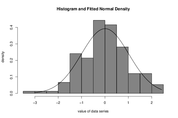
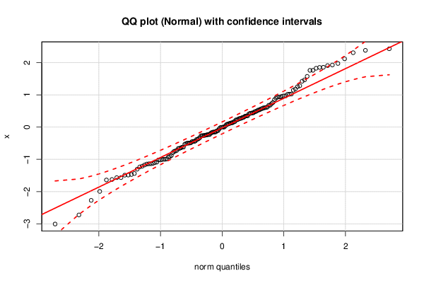
| Title produced by software | ML Fitting and QQ Plot- Normal Distribution | ||||||||||||||||||||||||||||||||||||||
| Date of computation | Sat, 21 Nov 2015 11:04:58 +0000 | ||||||||||||||||||||||||||||||||||||||
| Cite this page as follows | Statistical Computations at FreeStatistics.org, Office for Research Development and Education, URL https://freestatistics.org/blog/index.php?v=date/2015/Nov/21/t1448104146srnucsv23umajwk.htm/, Retrieved Tue, 14 May 2024 14:17:01 +0000 | ||||||||||||||||||||||||||||||||||||||
| Statistical Computations at FreeStatistics.org, Office for Research Development and Education, URL https://freestatistics.org/blog/index.php?pk=283747, Retrieved Tue, 14 May 2024 14:17:01 +0000 | |||||||||||||||||||||||||||||||||||||||
| QR Codes: | |||||||||||||||||||||||||||||||||||||||
|
| |||||||||||||||||||||||||||||||||||||||
| Original text written by user: | we kunnen zien in het histogram dat de kolommen zich grotendeels binnen de Gausscurve bevinden en we herkennen ook de "pyramide"-vorm van een normaalverdeling. | ||||||||||||||||||||||||||||||||||||||
| IsPrivate? | No (this computation is public) | ||||||||||||||||||||||||||||||||||||||
| User-defined keywords | |||||||||||||||||||||||||||||||||||||||
| Estimated Impact | 125 | ||||||||||||||||||||||||||||||||||||||
Tree of Dependent Computations | |||||||||||||||||||||||||||||||||||||||
| Family? (F = Feedback message, R = changed R code, M = changed R Module, P = changed Parameters, D = changed Data) | |||||||||||||||||||||||||||||||||||||||
| - [ML Fitting and QQ Plot- Normal Distribution] [3.1 task 3 ] [2015-11-21 11:04:58] [bfb327cc38fccc6d3daed2ac8fd9ce3b] [Current] | |||||||||||||||||||||||||||||||||||||||
| Feedback Forum | |||||||||||||||||||||||||||||||||||||||
Post a new message | |||||||||||||||||||||||||||||||||||||||
Dataset | |||||||||||||||||||||||||||||||||||||||
| Dataseries X: | |||||||||||||||||||||||||||||||||||||||
-0.112460901 -1.000359264 0.07540336765 -1.212361048 0.5994809383 -0.5134812403 0.09961817848 -0.2681705061 0.6207572576 0.4107303911 1.017084358 0.677832244 -0.3540277056 -0.2313521194 -0.8826560871 -1.123725843 -1.135920317 -0.6430683885 0.2990955021 0.529986936 0.3247154712 -0.6619179438 0.9599646381 0.1329963251 0.8514063703 -1.147133877 -1.566850218 1.856386339 -0.4983475379 0.6796196388 0.970942358 -1.018961665 1.573885363 0.9404233095 -2.724877613 -0.622754545 0.1613013208 -0.1458451057 0.5742291593 0.03120187756 1.252568951 0.5364159748 -0.752293437 -0.3816331102 -0.6205874997 -0.1536664948 -1.003076348 0.12370452 -0.1889302798 -0.7197629525 0.563070081 -1.491202585 0.2956249997 -1.087790287 -0.008073096656 0.4258361781 0.3482171228 2.381515657 0.4455116498 -0.02151612207 -0.9138775204 1.926901629 -1.439401004 -1.470384984 0.6107132434 -0.5322265364 0.3541165611 -0.4440701115 0.9362899003 -0.2677518031 -0.3245850206 -0.4505561733 1.465789638 0.4320806777 -0.7945862963 0.9658515317 -0.9866307645 0.4844652313 0.002621350644 0.2197663191 -1.626136871 1.280712522 0.5960312953 0.7268341727 0.4391161994 0.001801415959 -0.3751078294 -0.007276619974 -1.138807787 -1.019194541 1.025353331 -0.251011619 0.2624563181 0.1121949821 -1.236014557 0.1358093174 -3.007466636 2.308013447 2.11817579 0.9316060931 -1.567859058 -0.9990704298 -0.4966008483 -0.1704720284 -0.1562027708 -1.305836044 -0.1526370741 1.760817282 -0.2305959536 -0.4417091644 -0.4889722074 0.2650491534 1.974704858 -0.9250853569 -0.2434966668 1.907245613 -0.05938215783 -2.27277769 1.76181835 -0.2581351707 0.9014439297 -0.2625907214 1.182566536 -1.176334664 2.429949607 1.850981948 -0.7395732483 -0.2345546485 -0.4306748821 0.1679340328 0.4785588948 0.342656974 -1.487982543 1.020798434 0.7638740132 1.144895628 1.825438315 -1.100426105 0.2361800735 0.2742640192 0.2245470319 1.423526969 -0.4957975476 0.09061157434 -0.1086913321 -1.640131308 0.5084793192 -1.996351216 -0.6589728217 | |||||||||||||||||||||||||||||||||||||||
Tables (Output of Computation) | |||||||||||||||||||||||||||||||||||||||
| |||||||||||||||||||||||||||||||||||||||
Figures (Output of Computation) | |||||||||||||||||||||||||||||||||||||||
Input Parameters & R Code | |||||||||||||||||||||||||||||||||||||||
| Parameters (Session): | |||||||||||||||||||||||||||||||||||||||
| par1 = 8 ; par2 = 0 ; | |||||||||||||||||||||||||||||||||||||||
| Parameters (R input): | |||||||||||||||||||||||||||||||||||||||
| par1 = 8 ; par2 = 0 ; | |||||||||||||||||||||||||||||||||||||||
| R code (references can be found in the software module): | |||||||||||||||||||||||||||||||||||||||
library(MASS) | |||||||||||||||||||||||||||||||||||||||