Free Statistics
of Irreproducible Research!
Description of Statistical Computation | |||||||||||||||||||||||||||||||||||||||||||||||||||||||||||||||||||||||||||||||||||||||||||||||||||||||||||||||||||||||||||||||||||||||||||||||||||||||||||||||||||||||||||||||||||||||||||||||||||||||||||||||||||||||||||||||||||||||||||||||||||||||||||||||||||||||||||||||||||||||||||||||||||||||||||||||||||||||||
|---|---|---|---|---|---|---|---|---|---|---|---|---|---|---|---|---|---|---|---|---|---|---|---|---|---|---|---|---|---|---|---|---|---|---|---|---|---|---|---|---|---|---|---|---|---|---|---|---|---|---|---|---|---|---|---|---|---|---|---|---|---|---|---|---|---|---|---|---|---|---|---|---|---|---|---|---|---|---|---|---|---|---|---|---|---|---|---|---|---|---|---|---|---|---|---|---|---|---|---|---|---|---|---|---|---|---|---|---|---|---|---|---|---|---|---|---|---|---|---|---|---|---|---|---|---|---|---|---|---|---|---|---|---|---|---|---|---|---|---|---|---|---|---|---|---|---|---|---|---|---|---|---|---|---|---|---|---|---|---|---|---|---|---|---|---|---|---|---|---|---|---|---|---|---|---|---|---|---|---|---|---|---|---|---|---|---|---|---|---|---|---|---|---|---|---|---|---|---|---|---|---|---|---|---|---|---|---|---|---|---|---|---|---|---|---|---|---|---|---|---|---|---|---|---|---|---|---|---|---|---|---|---|---|---|---|---|---|---|---|---|---|---|---|---|---|---|---|---|---|---|---|---|---|---|---|---|---|---|---|---|---|---|---|---|---|---|---|---|---|---|---|---|---|---|---|---|---|---|---|---|---|---|---|---|---|---|---|---|---|---|---|---|---|---|---|---|---|---|---|---|---|---|---|---|---|---|---|---|---|---|---|---|---|
| Author's title | |||||||||||||||||||||||||||||||||||||||||||||||||||||||||||||||||||||||||||||||||||||||||||||||||||||||||||||||||||||||||||||||||||||||||||||||||||||||||||||||||||||||||||||||||||||||||||||||||||||||||||||||||||||||||||||||||||||||||||||||||||||||||||||||||||||||||||||||||||||||||||||||||||||||||||||||||||||||||
| Author | *Unverified author* | ||||||||||||||||||||||||||||||||||||||||||||||||||||||||||||||||||||||||||||||||||||||||||||||||||||||||||||||||||||||||||||||||||||||||||||||||||||||||||||||||||||||||||||||||||||||||||||||||||||||||||||||||||||||||||||||||||||||||||||||||||||||||||||||||||||||||||||||||||||||||||||||||||||||||||||||||||||||||
| R Software Module | rwasp_hierarchicalclustering.wasp | ||||||||||||||||||||||||||||||||||||||||||||||||||||||||||||||||||||||||||||||||||||||||||||||||||||||||||||||||||||||||||||||||||||||||||||||||||||||||||||||||||||||||||||||||||||||||||||||||||||||||||||||||||||||||||||||||||||||||||||||||||||||||||||||||||||||||||||||||||||||||||||||||||||||||||||||||||||||||
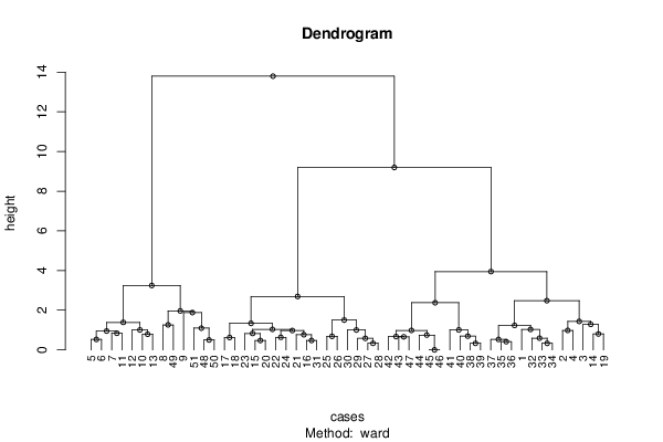
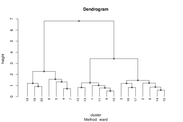
| Title produced by software | Hierarchical Clustering | ||||||||||||||||||||||||||||||||||||||||||||||||||||||||||||||||||||||||||||||||||||||||||||||||||||||||||||||||||||||||||||||||||||||||||||||||||||||||||||||||||||||||||||||||||||||||||||||||||||||||||||||||||||||||||||||||||||||||||||||||||||||||||||||||||||||||||||||||||||||||||||||||||||||||||||||||||||||||
| Date of computation | Thu, 19 Nov 2015 17:26:19 +0000 | ||||||||||||||||||||||||||||||||||||||||||||||||||||||||||||||||||||||||||||||||||||||||||||||||||||||||||||||||||||||||||||||||||||||||||||||||||||||||||||||||||||||||||||||||||||||||||||||||||||||||||||||||||||||||||||||||||||||||||||||||||||||||||||||||||||||||||||||||||||||||||||||||||||||||||||||||||||||||
| Cite this page as follows | Statistical Computations at FreeStatistics.org, Office for Research Development and Education, URL https://freestatistics.org/blog/index.php?v=date/2015/Nov/19/t1447954129ypfoap69srkbi89.htm/, Retrieved Tue, 14 May 2024 21:04:21 +0000 | ||||||||||||||||||||||||||||||||||||||||||||||||||||||||||||||||||||||||||||||||||||||||||||||||||||||||||||||||||||||||||||||||||||||||||||||||||||||||||||||||||||||||||||||||||||||||||||||||||||||||||||||||||||||||||||||||||||||||||||||||||||||||||||||||||||||||||||||||||||||||||||||||||||||||||||||||||||||||
| Statistical Computations at FreeStatistics.org, Office for Research Development and Education, URL https://freestatistics.org/blog/index.php?pk=283661, Retrieved Tue, 14 May 2024 21:04:21 +0000 | |||||||||||||||||||||||||||||||||||||||||||||||||||||||||||||||||||||||||||||||||||||||||||||||||||||||||||||||||||||||||||||||||||||||||||||||||||||||||||||||||||||||||||||||||||||||||||||||||||||||||||||||||||||||||||||||||||||||||||||||||||||||||||||||||||||||||||||||||||||||||||||||||||||||||||||||||||||||||
| QR Codes: | |||||||||||||||||||||||||||||||||||||||||||||||||||||||||||||||||||||||||||||||||||||||||||||||||||||||||||||||||||||||||||||||||||||||||||||||||||||||||||||||||||||||||||||||||||||||||||||||||||||||||||||||||||||||||||||||||||||||||||||||||||||||||||||||||||||||||||||||||||||||||||||||||||||||||||||||||||||||||
|
| |||||||||||||||||||||||||||||||||||||||||||||||||||||||||||||||||||||||||||||||||||||||||||||||||||||||||||||||||||||||||||||||||||||||||||||||||||||||||||||||||||||||||||||||||||||||||||||||||||||||||||||||||||||||||||||||||||||||||||||||||||||||||||||||||||||||||||||||||||||||||||||||||||||||||||||||||||||||||
| Original text written by user: | |||||||||||||||||||||||||||||||||||||||||||||||||||||||||||||||||||||||||||||||||||||||||||||||||||||||||||||||||||||||||||||||||||||||||||||||||||||||||||||||||||||||||||||||||||||||||||||||||||||||||||||||||||||||||||||||||||||||||||||||||||||||||||||||||||||||||||||||||||||||||||||||||||||||||||||||||||||||||
| IsPrivate? | No (this computation is public) | ||||||||||||||||||||||||||||||||||||||||||||||||||||||||||||||||||||||||||||||||||||||||||||||||||||||||||||||||||||||||||||||||||||||||||||||||||||||||||||||||||||||||||||||||||||||||||||||||||||||||||||||||||||||||||||||||||||||||||||||||||||||||||||||||||||||||||||||||||||||||||||||||||||||||||||||||||||||||
| User-defined keywords | |||||||||||||||||||||||||||||||||||||||||||||||||||||||||||||||||||||||||||||||||||||||||||||||||||||||||||||||||||||||||||||||||||||||||||||||||||||||||||||||||||||||||||||||||||||||||||||||||||||||||||||||||||||||||||||||||||||||||||||||||||||||||||||||||||||||||||||||||||||||||||||||||||||||||||||||||||||||||
| Estimated Impact | 73 | ||||||||||||||||||||||||||||||||||||||||||||||||||||||||||||||||||||||||||||||||||||||||||||||||||||||||||||||||||||||||||||||||||||||||||||||||||||||||||||||||||||||||||||||||||||||||||||||||||||||||||||||||||||||||||||||||||||||||||||||||||||||||||||||||||||||||||||||||||||||||||||||||||||||||||||||||||||||||
Tree of Dependent Computations | |||||||||||||||||||||||||||||||||||||||||||||||||||||||||||||||||||||||||||||||||||||||||||||||||||||||||||||||||||||||||||||||||||||||||||||||||||||||||||||||||||||||||||||||||||||||||||||||||||||||||||||||||||||||||||||||||||||||||||||||||||||||||||||||||||||||||||||||||||||||||||||||||||||||||||||||||||||||||
| Family? (F = Feedback message, R = changed R code, M = changed R Module, P = changed Parameters, D = changed Data) | |||||||||||||||||||||||||||||||||||||||||||||||||||||||||||||||||||||||||||||||||||||||||||||||||||||||||||||||||||||||||||||||||||||||||||||||||||||||||||||||||||||||||||||||||||||||||||||||||||||||||||||||||||||||||||||||||||||||||||||||||||||||||||||||||||||||||||||||||||||||||||||||||||||||||||||||||||||||||
| - [Hierarchical Clustering] [Rodolfo 50] [2015-11-19 17:26:19] [d41d8cd98f00b204e9800998ecf8427e] [Current] | |||||||||||||||||||||||||||||||||||||||||||||||||||||||||||||||||||||||||||||||||||||||||||||||||||||||||||||||||||||||||||||||||||||||||||||||||||||||||||||||||||||||||||||||||||||||||||||||||||||||||||||||||||||||||||||||||||||||||||||||||||||||||||||||||||||||||||||||||||||||||||||||||||||||||||||||||||||||||
| Feedback Forum | |||||||||||||||||||||||||||||||||||||||||||||||||||||||||||||||||||||||||||||||||||||||||||||||||||||||||||||||||||||||||||||||||||||||||||||||||||||||||||||||||||||||||||||||||||||||||||||||||||||||||||||||||||||||||||||||||||||||||||||||||||||||||||||||||||||||||||||||||||||||||||||||||||||||||||||||||||||||||
Post a new message | |||||||||||||||||||||||||||||||||||||||||||||||||||||||||||||||||||||||||||||||||||||||||||||||||||||||||||||||||||||||||||||||||||||||||||||||||||||||||||||||||||||||||||||||||||||||||||||||||||||||||||||||||||||||||||||||||||||||||||||||||||||||||||||||||||||||||||||||||||||||||||||||||||||||||||||||||||||||||
Dataset | |||||||||||||||||||||||||||||||||||||||||||||||||||||||||||||||||||||||||||||||||||||||||||||||||||||||||||||||||||||||||||||||||||||||||||||||||||||||||||||||||||||||||||||||||||||||||||||||||||||||||||||||||||||||||||||||||||||||||||||||||||||||||||||||||||||||||||||||||||||||||||||||||||||||||||||||||||||||||
| Dataseries X: | |||||||||||||||||||||||||||||||||||||||||||||||||||||||||||||||||||||||||||||||||||||||||||||||||||||||||||||||||||||||||||||||||||||||||||||||||||||||||||||||||||||||||||||||||||||||||||||||||||||||||||||||||||||||||||||||||||||||||||||||||||||||||||||||||||||||||||||||||||||||||||||||||||||||||||||||||||||||||
0.33 0.50 0.00 0.25 0.00 0.00 0.33 0.25 0.50 1.00 0.33 0.33 1.00 1.00 0.00 0.00 0.66 0.50 0.00 0.66 0.75 0.33 0.75 0.75 0.50 0.75 0.66 0.33 0.66 0.66 0.33 0.33 0.66 0.50 0.75 0.25 0.25 0.33 0.75 0.50 0.50 0.33 0.33 0.75 1.00 0.75 0.33 0.75 0.33 0.50 0.00 0.25 0.50 0.66 0.66 0.50 0.50 0.66 0.33 0.66 0.33 0.66 0.33 0.00 0.66 1.00 0.66 0.66 0.75 0.66 0.66 0.75 1.00 0.66 0.33 0.66 0.33 0.66 0.66 0.66 0.66 1.00 0.66 0.66 0.50 0.66 0.66 0.75 1.00 0.66 0.33 0.66 0.33 0.66 0.33 0.33 1.00 1.00 0.66 0.66 0.75 0.66 0.66 0.75 1.00 1.00 0.66 0.66 0.33 0.66 0.66 1.00 1.00 0.00 1.00 1.00 0.75 0.66 0.66 0.75 1.00 1.00 0.66 0.66 0.33 0.66 0.66 0.66 1.00 1.00 1.00 1.00 1.00 0.66 0.66 1.00 0.00 1.00 1.00 1.00 0.33 0.66 1.00 1.00 0.66 1.00 0.66 0.66 0.75 0.66 0.66 0.75 0.50 0.66 0.33 0.33 0.66 1.00 0.66 0.66 0.66 1.00 1.00 1.00 1.00 0.66 0.66 1.00 1.00 0.66 0.66 0.66 0.33 0.66 0.66 0.66 0.66 1.00 1.00 0.66 1.00 0.66 0.25 0.75 0.50 0.66 0.66 0.66 0.66 0.66 0.66 0.33 0.66 1.00 0.66 0.66 0.75 0.66 0.75 0.50 0.50 0.33 0.33 0.33 0.33 0.66 0.33 0.33 0.25 0.50 0.66 0.33 0.50 0.33 0.66 0.50 0.50 0.66 0.66 0.33 0.66 0.33 0.33 0.33 0.33 0.50 0.33 0.33 0.00 0.33 0.33 0.33 0.50 1.00 0.00 0.00 1.00 0.33 0.00 0.00 0.33 0.50 0.33 0.33 0.33 0.33 0.33 0.33 0.50 1.00 0.33 0.33 0.66 0.33 0.00 0.00 0.33 1.00 0.33 0.33 0.00 0.33 0.33 0.25 0.50 0.66 0.00 0.33 0.66 0.33 0.00 0.00 0.33 1.00 0.33 0.33 0.25 0.33 0.33 0.25 0.50 0.66 0.33 0.33 0.66 0.66 0.33 0.00 0.33 0.00 0.66 0.33 0.25 0.33 0.33 0.50 0.50 0.66 0.66 0.33 0.66 0.66 0.33 0.00 0.33 0.50 0.33 0.33 0.00 0.33 0.33 0.25 0.50 1.00 0.00 0.33 1.00 0.33 0.33 0.00 0.25 0.50 0.33 0.33 0.00 0.33 0.33 0.25 0.00 1.00 0.33 0.33 0.66 0.33 0.33 0.00 0.25 0.50 0.66 0.33 0.33 0.00 0.33 0.25 0.50 1.00 0.33 0.33 1.00 0.33 0.00 0.00 0.00 0.50 0.33 0.00 0.00 0.00 0.33 0.25 0.50 1.00 0.00 0.33 1.00 0.00 0.00 0.00 0.33 0.50 0.66 0.00 0.33 0.33 0.33 0.50 0.50 0.66 0.33 0.33 1.00 0.33 0.00 0.00 0.00 0.50 0.33 0.00 0.00 0.00 0.00 0.33 0.50 0.66 0.33 0.00 1.00 0.00 0.33 0.00 0.00 0.50 0.00 0.00 0.00 0.00 0.33 0.33 0.00 0.66 0.33 0.00 1.00 0.00 0.33 0.00 0.00 0.00 0.00 0.00 0.00 0.00 0.33 0.25 0.50 1.00 0.33 0.00 0.66 0.33 0.00 0.00 0.00 0.00 0.00 0.00 0.00 0.00 0.33 0.25 0.50 1.00 0.33 0.00 0.66 0.00 0.00 0.00 0.00 0.00 0.00 0.33 0.00 0.00 0.33 0.25 0.50 1.00 0.00 0.00 0.66 0.33 0.00 0.00 0.00 0.50 0.00 0.33 0.00 0.00 0.33 0.25 0.00 1.00 0.00 0.00 0.66 0.33 0.00 0.00 0.33 0.50 0.33 0.00 0.00 0.33 0.33 0.25 0.50 1.00 0.33 0.33 0.66 0.33 0.00 0.00 0.33 0.50 0.33 0.00 0.00 0.33 0.33 0.25 0.50 1.00 0.66 0.33 0.66 0.66 0.00 0.33 0.33 0.50 0.33 0.33 0.00 0.33 0.33 0.25 0.50 1.00 0.66 0.33 1.00 0.66 0.33 0.33 0.33 0.50 0.33 0.00 0.00 0.33 0.33 0.25 0.50 1.00 0.66 0.33 1.00 0.66 0.33 0.33 0.33 0.50 0.33 0.33 0.00 0.33 0.33 0.25 0.50 1.00 0.66 0.66 1.00 0.66 0.33 0.00 0.33 0.50 0.66 0.33 0.00 0.33 0.33 0.50 0.50 1.00 0.66 0.66 1.00 0.66 0.33 0.00 0.33 0.50 0.66 0.00 0.25 0.33 0.33 0.50 0.50 1.00 0.66 0.66 1.00 0.66 0.33 0.00 0.66 0.50 0.33 0.00 0.25 0.33 0.66 0.50 0.50 1.00 1.00 1.00 1.00 0.66 0.33 0.33 0.66 0.50 0.33 0.00 0.25 0.33 0.33 0.50 0.50 1.00 1.00 1.00 1.00 0.66 0.33 0.33 0.66 0.50 0.33 0.00 0.25 0.33 0.00 0.50 0.50 1.00 1.00 1.00 1.00 0.66 0.33 0.66 0.33 0.00 0.33 0.00 0.00 0.33 0.33 0.33 0.50 1.00 1.00 1.00 1.00 1.00 0.33 0.66 0.66 0.50 0.66 0.33 0.25 0.33 0.33 0.50 0.50 1.00 1.00 1.00 0.66 1.00 0.66 0.66 0.66 0.50 0.66 0.33 0.25 0.33 0.66 0.50 0.50 1.00 1.00 0.66 1.00 1.00 0.66 0.33 0.33 1.00 0.66 0.33 0.25 0.33 0.66 0.50 0.50 1.00 1.00 0.66 0.66 1.00 0.66 0.66 0.33 0.50 0.66 0.33 0.25 0.33 0.66 0.75 0.50 1.00 1.00 0.66 0.66 1.00 0.66 0.66 0.33 0.50 0.66 0.33 0.25 0.33 0.66 0.75 0.50 1.00 1.00 0.66 0.66 1.00 0.66 0.66 0.33 0.50 0.66 0.33 0.25 0.66 0.33 0.50 0.50 1.00 1.00 0.66 1.00 1.00 0.66 0.66 0.33 1.00 0.66 0.66 0.50 0.66 0.66 0.75 0.50 1.00 1.00 1.00 1.00 1.00 0.66 1.00 0.33 0.00 0.66 0.66 0.75 0.66 0.66 0.75 1.00 1.00 1.00 1.00 1.00 1.00 0.66 1.00 0.33 1.00 0.66 0.66 0.50 0.66 0.66 0.75 1.00 1.00 1.00 1.00 1.00 1.00 0.66 1.00 0.33 1.00 1.00 1.00 1.00 1.00 1.00 1.00 1.00 1.00 1.00 1.00 1.00 1.00 0.66 1.00 | |||||||||||||||||||||||||||||||||||||||||||||||||||||||||||||||||||||||||||||||||||||||||||||||||||||||||||||||||||||||||||||||||||||||||||||||||||||||||||||||||||||||||||||||||||||||||||||||||||||||||||||||||||||||||||||||||||||||||||||||||||||||||||||||||||||||||||||||||||||||||||||||||||||||||||||||||||||||||
Tables (Output of Computation) | |||||||||||||||||||||||||||||||||||||||||||||||||||||||||||||||||||||||||||||||||||||||||||||||||||||||||||||||||||||||||||||||||||||||||||||||||||||||||||||||||||||||||||||||||||||||||||||||||||||||||||||||||||||||||||||||||||||||||||||||||||||||||||||||||||||||||||||||||||||||||||||||||||||||||||||||||||||||||
| |||||||||||||||||||||||||||||||||||||||||||||||||||||||||||||||||||||||||||||||||||||||||||||||||||||||||||||||||||||||||||||||||||||||||||||||||||||||||||||||||||||||||||||||||||||||||||||||||||||||||||||||||||||||||||||||||||||||||||||||||||||||||||||||||||||||||||||||||||||||||||||||||||||||||||||||||||||||||
Figures (Output of Computation) | |||||||||||||||||||||||||||||||||||||||||||||||||||||||||||||||||||||||||||||||||||||||||||||||||||||||||||||||||||||||||||||||||||||||||||||||||||||||||||||||||||||||||||||||||||||||||||||||||||||||||||||||||||||||||||||||||||||||||||||||||||||||||||||||||||||||||||||||||||||||||||||||||||||||||||||||||||||||||
Input Parameters & R Code | |||||||||||||||||||||||||||||||||||||||||||||||||||||||||||||||||||||||||||||||||||||||||||||||||||||||||||||||||||||||||||||||||||||||||||||||||||||||||||||||||||||||||||||||||||||||||||||||||||||||||||||||||||||||||||||||||||||||||||||||||||||||||||||||||||||||||||||||||||||||||||||||||||||||||||||||||||||||||
| Parameters (Session): | |||||||||||||||||||||||||||||||||||||||||||||||||||||||||||||||||||||||||||||||||||||||||||||||||||||||||||||||||||||||||||||||||||||||||||||||||||||||||||||||||||||||||||||||||||||||||||||||||||||||||||||||||||||||||||||||||||||||||||||||||||||||||||||||||||||||||||||||||||||||||||||||||||||||||||||||||||||||||
| par1 = ward ; par2 = 20 ; par3 = FALSE ; par4 = FALSE ; | |||||||||||||||||||||||||||||||||||||||||||||||||||||||||||||||||||||||||||||||||||||||||||||||||||||||||||||||||||||||||||||||||||||||||||||||||||||||||||||||||||||||||||||||||||||||||||||||||||||||||||||||||||||||||||||||||||||||||||||||||||||||||||||||||||||||||||||||||||||||||||||||||||||||||||||||||||||||||
| Parameters (R input): | |||||||||||||||||||||||||||||||||||||||||||||||||||||||||||||||||||||||||||||||||||||||||||||||||||||||||||||||||||||||||||||||||||||||||||||||||||||||||||||||||||||||||||||||||||||||||||||||||||||||||||||||||||||||||||||||||||||||||||||||||||||||||||||||||||||||||||||||||||||||||||||||||||||||||||||||||||||||||
| par1 = ward ; par2 = 20 ; par3 = FALSE ; par4 = FALSE ; | |||||||||||||||||||||||||||||||||||||||||||||||||||||||||||||||||||||||||||||||||||||||||||||||||||||||||||||||||||||||||||||||||||||||||||||||||||||||||||||||||||||||||||||||||||||||||||||||||||||||||||||||||||||||||||||||||||||||||||||||||||||||||||||||||||||||||||||||||||||||||||||||||||||||||||||||||||||||||
| R code (references can be found in the software module): | |||||||||||||||||||||||||||||||||||||||||||||||||||||||||||||||||||||||||||||||||||||||||||||||||||||||||||||||||||||||||||||||||||||||||||||||||||||||||||||||||||||||||||||||||||||||||||||||||||||||||||||||||||||||||||||||||||||||||||||||||||||||||||||||||||||||||||||||||||||||||||||||||||||||||||||||||||||||||
par4 <- 'FALSE' | |||||||||||||||||||||||||||||||||||||||||||||||||||||||||||||||||||||||||||||||||||||||||||||||||||||||||||||||||||||||||||||||||||||||||||||||||||||||||||||||||||||||||||||||||||||||||||||||||||||||||||||||||||||||||||||||||||||||||||||||||||||||||||||||||||||||||||||||||||||||||||||||||||||||||||||||||||||||||