Repository of Reproducible Computations

Free Statistics

of Irreproducible Research!

Author's title

Author

*The author of this computation has been verified*

R Software Module

rwasp_fitdistrnorm.wasp

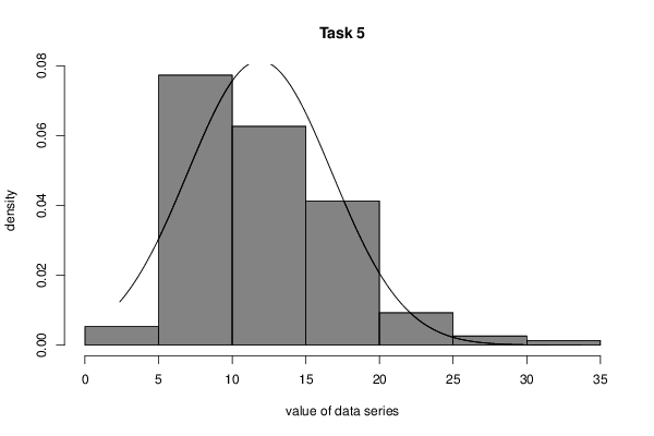
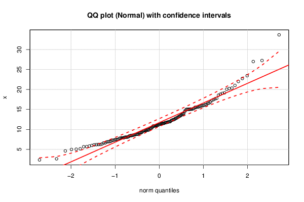
Title produced by software

ML Fitting and QQ Plot- Normal Distribution

Date of computation

Mon, 16 Nov 2015 11:57:45 +0000

Cite this page as follows

Statistical Computations at FreeStatistics.org, Office for Research Development and Education, URL https://freestatistics.org/blog/index.php?v=date/2015/Nov/16/t1447675208fqueubwuj41mrxn.htm/, Retrieved Wed, 15 May 2024 04:44:20 +0000

Statistical Computations at FreeStatistics.org, Office for Research Development and Education, URL https://freestatistics.org/blog/index.php?pk=283358, Retrieved Wed, 15 May 2024 04:44:20 +0000

QR Codes:

Paste this QR Code to cite your computation.

Original text written by user:

IsPrivate?

No (this computation is public)

User-defined keywords

Estimated Impact

103

Family? (F = Feedback message, R = changed R code, M = changed R Module, P = changed Parameters, D = changed Data)

-       [ML Fitting and QQ Plot- Normal Distribution] [Task 5 problem 2] [2015-11-16 11:57:45] [024df7c298481a95aca593c6dd9022cb] [Current]

Feedback Forum

Post a new message

Dataseries X:

Download CSV

Histogram

Boxplots

7.511313209
9.192026731
10.85283232
21.99609818
9.844448102
5.684108002
7.885767608
9.839193691
9.074919587
11.94388435
15.94342318
8.043623703
13.78289517
4.616491195
12.55608274
4.982655978
17.79582648
5.044985207
8.206527354
8.61281972
7.289526959
8.432901538
18.80752256
5.986755454
15.69383338
16.85733517
11.30637523
9.602020144
10.33925673
5.148866276
15.53282743
11.38389642
5.661801497
11.77662831
27.25144577
9.6740419
19.15874831
12.12687228
6.952506776
6.181022161
14.46352913
20.23067985
11.52007221
7.819781982
6.615394277
16.17046609
11.02161428
8.081371853
22.74864744
6.141747076
13.03526905
12.32578968
16.58750428
8.688889397
13.86212725
15.0275242
10.84684061
2.639125598
9.69888751
12.31014746
8.075225055
15.51812723
5.832723396
12.79165036
7.893590789
10.96049367
10.22996422
11.21708478
8.385985281
8.568669747
7.292529828
9.72118583
9.70808882
11.72325313
11.65372402
11.9320012
11.09547693
17.45863372
13.20200332
12.44750862
12.46884456
19.01779513
11.53690815
15.15822384
11.48834689
9.918432012
15.07140114
9.201249304
9.397069495
8.500891182
8.731151168
15.05050068
13.41253402
13.54378977
8.821737871
11.89453796
6.920982511
15.84812178
10.4961099
11.84636559
16.20183227
6.605378339
9.846593441
16.52250489
7.400680262
15.02927973
6.328979126
11.49771679
23.44485354
13.9479707
11.38813464
21.01052618
20.04680218
6.879338209
15.01467779
10.92646766
8.451439159
7.438357151
18.56405427
15.59725236
17.27246613
8.788613352
10.82963186
8.057865967
17.66118851
7.4807578
7.770195465
15.22783323
6.220258679
10.89617753
15.07222938
9.177485968
10.25885502
15.0140342
11.70213514
13.32894365
7.890281751
15.89326
33.67918046
16.03883943
7.045817922
12.79450057
8.796606798
2.367071828
6.234107245
14.77150784
26.98964639
20.35077644
12.93596537
15.60427325

Summary of computational transaction
Raw Input	view raw input (R code)
Raw Output	view raw output of R engine
Computing time	4 seconds
R Server	'Gwilym Jenkins' @ jenkins.wessa.net

\begin{tabular}{lllllllll}
\hline
Summary of computational transaction \tabularnewline
Raw Input & view raw input (R code)  \tabularnewline
Raw Output & view raw output of R engine  \tabularnewline
Computing time & 4 seconds \tabularnewline
R Server & 'Gwilym Jenkins' @ jenkins.wessa.net \tabularnewline
\hline
\end{tabular}
%Source: https://freestatistics.org/blog/index.php?pk=283358&T=0

[TABLE]
[ROW][C]Summary of computational transaction[/C][/ROW]
[ROW][C]Raw Input[/C][C]view raw input (R code) [/C][/ROW]
[ROW][C]Raw Output[/C][C]view raw output of R engine [/C][/ROW]
[ROW][C]Computing time[/C][C]4 seconds[/C][/ROW]
[ROW][C]R Server[/C][C]'Gwilym Jenkins' @ jenkins.wessa.net[/C][/ROW]
[/TABLE]
Source: https://freestatistics.org/blog/index.php?pk=283358&T=0

Globally Unique Identifier (entire table): ba.freestatistics.org/blog/index.php?pk=283358&T=0

As an alternative you can also use a QR Code:

The GUIDs for individual cells are displayed in the table below:

Summary of computational transaction
Raw Input	view raw input (R code)
Raw Output	view raw output of R engine
Computing time	4 seconds
R Server	'Gwilym Jenkins' @ jenkins.wessa.net

Parameter	Estimated Value	Standard Deviation
mean	11.8715718319067	0.399966889420007
standard deviation	4.89857396543601	0.282819299758977

\begin{tabular}{lllllllll}
\hline
Parameter & Estimated Value & Standard Deviation \tabularnewline
mean & 11.8715718319067 & 0.399966889420007 \tabularnewline
standard deviation & 4.89857396543601 & 0.282819299758977 \tabularnewline
\hline
\end{tabular}
%Source: https://freestatistics.org/blog/index.php?pk=283358&T=1

[TABLE]
[ROW][C]Parameter[/C][C]Estimated Value[/C][C]Standard Deviation[/C][/ROW]
[ROW][C]mean[/C][C]11.8715718319067[/C][C]0.399966889420007[/C][/ROW]
[ROW][C]standard deviation[/C][C]4.89857396543601[/C][C]0.282819299758977[/C][/ROW]
[/TABLE]
Source: https://freestatistics.org/blog/index.php?pk=283358&T=1

Globally Unique Identifier (entire table): ba.freestatistics.org/blog/index.php?pk=283358&T=1

As an alternative you can also use a QR Code:

The GUIDs for individual cells are displayed in the table below:

Parameter	Estimated Value	Standard Deviation
mean	11.8715718319067	0.399966889420007
standard deviation	4.89857396543601	0.282819299758977

Figure 1

PNG link

Postscript link

PDF link

Figure 2

PNG link

Postscript link

PDF link

Parameters (Session):

par1 = 8 ; par2 = 0 ;

Parameters (R input):

par1 = 8 ; par2 = 0 ;

R code (references can be found in the software module):

library(MASS)
library(car)
par1 <- as.numeric(par1)
if (par2 == '0') par2 = 'Sturges' else par2 <- as.numeric(par2)
x <- as.ts(x) #otherwise the fitdistr function does not work properly
r <- fitdistr(x,'normal')
r
bitmap(file='test1.png')
myhist<-hist(x,col=par1,breaks=par2,main=main,ylab=ylab,xlab=xlab,freq=F)
curve(1/(r$estimate[2]*sqrt(2*pi))*exp(-1/2*((x-r$estimate[1])/r$estimate[2])^2),min(x),max(x),add=T)
dev.off()
bitmap(file='test3.png')
qqPlot(x,dist='norm',main='QQ plot (Normal) with confidence intervals')
grid()
dev.off()
load(file='createtable')
a<-table.start()
a<-table.row.start(a)
a<-table.element(a,'Parameter',1,TRUE)
a<-table.element(a,'Estimated Value',1,TRUE)
a<-table.element(a,'Standard Deviation',1,TRUE)
a<-table.row.end(a)
a<-table.row.start(a)
a<-table.element(a,'mean',header=TRUE)
a<-table.element(a,r$estimate[1])
a<-table.element(a,r$sd[1])
a<-table.row.end(a)
a<-table.row.start(a)
a<-table.element(a,'standard deviation',header=TRUE)
a<-table.element(a,r$estimate[2])
a<-table.element(a,r$sd[2])
a<-table.row.end(a)
a<-table.end(a)
table.save(a,file='mytable.tab')

Free Statistics

Description of Statistical Computation

Tree of Dependent Computations

Dataset

Tables (Output of Computation)

Figures (Output of Computation)

Input Parameters & R Code