Free Statistics
of Irreproducible Research!
Description of Statistical Computation | |||||||||||||||||||||||||||||||||||||||
|---|---|---|---|---|---|---|---|---|---|---|---|---|---|---|---|---|---|---|---|---|---|---|---|---|---|---|---|---|---|---|---|---|---|---|---|---|---|---|---|
| Author's title | |||||||||||||||||||||||||||||||||||||||
| Author | *The author of this computation has been verified* | ||||||||||||||||||||||||||||||||||||||
| R Software Module | rwasp_fitdistrnorm.wasp | ||||||||||||||||||||||||||||||||||||||
| Title produced by software | ML Fitting and QQ Plot- Normal Distribution | ||||||||||||||||||||||||||||||||||||||
| Date of computation | Sat, 07 Nov 2015 22:27:31 +0000 | ||||||||||||||||||||||||||||||||||||||
| Cite this page as follows | Statistical Computations at FreeStatistics.org, Office for Research Development and Education, URL https://freestatistics.org/blog/index.php?v=date/2015/Nov/07/t14469353635nypvjqhfvvftoq.htm/, Retrieved Thu, 03 Jul 2025 19:49:55 +0000 | ||||||||||||||||||||||||||||||||||||||
| Statistical Computations at FreeStatistics.org, Office for Research Development and Education, URL https://freestatistics.org/blog/index.php?pk=283242, Retrieved Thu, 03 Jul 2025 19:49:55 +0000 | |||||||||||||||||||||||||||||||||||||||
| QR Codes: | |||||||||||||||||||||||||||||||||||||||
|
| |||||||||||||||||||||||||||||||||||||||
| Original text written by user: | |||||||||||||||||||||||||||||||||||||||
| IsPrivate? | No (this computation is public) | ||||||||||||||||||||||||||||||||||||||
| User-defined keywords | |||||||||||||||||||||||||||||||||||||||
| Estimated Impact | 195 | ||||||||||||||||||||||||||||||||||||||
Tree of Dependent Computations | |||||||||||||||||||||||||||||||||||||||
| Family? (F = Feedback message, R = changed R code, M = changed R Module, P = changed Parameters, D = changed Data) | |||||||||||||||||||||||||||||||||||||||
| - [ML Fitting and QQ Plot- Normal Distribution] [] [2015-09-28 10:11:33] [32b17a345b130fdf5cc88718ed94a974] - PD [ML Fitting and QQ Plot- Normal Distribution] [taak 4 h3 ] [2015-11-07 22:27:31] [f0540685e8d53548e4baf07e0669deea] [Current] | |||||||||||||||||||||||||||||||||||||||
| Feedback Forum | |||||||||||||||||||||||||||||||||||||||
Post a new message | |||||||||||||||||||||||||||||||||||||||
Dataset | |||||||||||||||||||||||||||||||||||||||
| Dataseries X: | |||||||||||||||||||||||||||||||||||||||
8.886868947 9.672102265 7.53576823 12.52225581 5.989517766 10.15568011 17.44597005 16.53644941 5.368395086 11.78967872 10.50560959 3.59515805 11.49663818 15.02554882 7.343499198 19.58510635 22.29473323 10.31588098 14.82303398 9.73971542 8.436943741 15.79918796 20.40295902 14.08741144 14.89823271 17.29760432 17.33653124 4.795611761 7.237536092 6.693064801 9.247527441 15.62053536 5.007679029 6.148742757 25.36981889 13.91771067 16.63174892 8.71051166 13.97360288 10.18692039 7.844937275 6.18031705 10.39697102 10.60433772 21.21647392 7.119257483 9.655455527 15.94655802 12.98753947 22.05627038 15.30440467 17.46326088 8.406890563 12.43066396 16.25873599 6.877443596 15.44013475 2.033286063 9.143107054 8.032586586 14.07594704 5.04918919 22.1215538 16.18506878 11.91460551 15.07750685 25.45649564 13.463028 10.13566869 13.39701868 10.42350089 13.95122375 5.783049422 8.730700855 17.41393105 5.430957626 11.02481355 11.54509623 15.15393002 10.36951819 28.97295202 11.38186067 6.110652845 10.78139469 10.13026922 19.38841748 14.65321955 11.90818066 14.31889705 14.12895652 4.059021333 12.86973495 14.05768449 9.236454793 9.48639237 12.46746251 21.23482356 5.92627398 6.795576262 6.813334494 15.51901138 16.49597449 15.84029831 6.517722983 7.165672986 12.56689993 12.70840272 6.8492796 8.076713636 19.52462591 12.49654214 8.685727591 3.852509454 12.55644862 11.03156083 12.89664109 8.837270741 21.51128057 6.648348318 18.14978076 17.6501806 17.20090618 6.991450269 10.73990575 6.210779039 7.192177997 13.29735435 11.98625592 10.61115113 19.88030949 16.34430915 5.201557722 17.5358452 6.818133913 10.73974911 6.862726768 7.560305296 13.22048125 11.26736775 4.205940475 14.44264419 7.569796063 8.194279072 12.30006224 12.08975817 19.59928525 13.32806195 19.96851337 16.79019159 | |||||||||||||||||||||||||||||||||||||||
Tables (Output of Computation) | |||||||||||||||||||||||||||||||||||||||
| |||||||||||||||||||||||||||||||||||||||
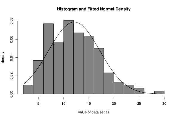
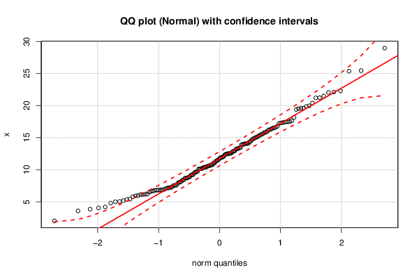
Figures (Output of Computation) | |||||||||||||||||||||||||||||||||||||||
Input Parameters & R Code | |||||||||||||||||||||||||||||||||||||||
| Parameters (Session): | |||||||||||||||||||||||||||||||||||||||
| Parameters (R input): | |||||||||||||||||||||||||||||||||||||||
| par1 = 8 ; par2 = 12 ; | |||||||||||||||||||||||||||||||||||||||
| R code (references can be found in the software module): | |||||||||||||||||||||||||||||||||||||||
library(MASS) | |||||||||||||||||||||||||||||||||||||||