Repository of Reproducible Computations

Free Statistics

of Irreproducible Research!

Author's title

Author

*The author of this computation has been verified*

R Software Module

rwasp_fitdistrnorm.wasp

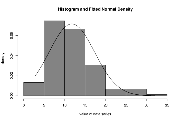
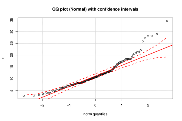
Title produced by software

ML Fitting and QQ Plot- Normal Distribution

Date of computation

Sat, 07 Nov 2015 16:44:50 +0000

Cite this page as follows

Statistical Computations at FreeStatistics.org, Office for Research Development and Education, URL https://freestatistics.org/blog/index.php?v=date/2015/Nov/07/t1446915098zxdjk5ddizeo021.htm/, Retrieved Tue, 14 May 2024 14:26:55 +0000

Statistical Computations at FreeStatistics.org, Office for Research Development and Education, URL https://freestatistics.org/blog/index.php?pk=283236, Retrieved Tue, 14 May 2024 14:26:55 +0000

QR Codes:

Paste this QR Code to cite your computation.

Original text written by user:

IsPrivate?

No (this computation is public)

User-defined keywords

Estimated Impact

152

Family? (F = Feedback message, R = changed R code, M = changed R Module, P = changed Parameters, D = changed Data)

-     [ML Fitting and QQ Plot- Normal Distribution] [Chapter 3 - Task 3] [2015-11-07 16:09:05] [74be16979710d4c4e7c6647856088456]
- R  D    [ML Fitting and QQ Plot- Normal Distribution] [Chapter 3 - Task ...] [2015-11-07 16:44:50] [024df7c298481a95aca593c6dd9022cb] [Current]

Feedback Forum

Post a new message

Dataseries X:

Download CSV

Histogram

Boxplots

11.8936928
9.281015548
3.072943269
10.97969874
18.11836282
3.580586696
5.917816243
17.55559388
9.410480678
3.750505849
16.71033913
11.96534392
6.530328715
11.18751006
7.861760714
18.47112898
6.024993051
20.88621553
7.693618298
4.866283315
20.64764579
7.482601722
12.12587508
8.692277381
10.32642404
10.4831548
13.28108781
10.81676345
8.257963072
7.029542553
9.161918172
5.076744847
14.2105606
21.31744768
10.03649573
9.151516493
7.010421195
25.81473485
12.81162729
6.785134407
14.16000347
8.743419105
5.766219498
9.945624481
12.10200612
12.27912242
8.610419949
8.733365043
9.554793778
14.8685502
9.393339325
10.90354067
10.42989819
13.89223336
2.86296658
13.04594117
8.191489207
15.39688535
7.660686564
8.22692413
7.428367521
4.654442493
4.678594788
10.56856857
14.77726316
2.760645869
9.659025033
17.43354388
34.568245
9.459012035
10.9158278
8.893135734
8.291318594
6.019593288
15.63453178
12.21572529
11.53612763
17.17599373
8.385161686
10.71498715
11.55199942
8.039574529
12.5378375
12.97441396
6.7779942
13.66985513
5.269821943
12.98065563
8.658388186
16.91660713
9.340083977
13.17265746
17.26804211
18.28451717
10.13710627
22.10512644
12.11148156
18.49967953
15.53359337
16.50376167
6.201882815
8.47568263
10.36215544
6.777214556
28.90806689
11.44956012
11.99679308
19.13622557
10.1731037
3.858395623
17.34665613
16.21209554
16.28886596
7.978158383
12.09360989
8.187085815
6.698517123
11.6901414
19.92325482
12.74284216
7.370057962
9.902442827
10.62188738
8.100149229
8.22502194
13.33914007
10.55351253
3.882367629
7.569254886
18.40027625
18.3850025
21.26252919
14.64622877
17.2542326
12.768092
9.571003817
12.50358249
9.875667315
7.227809811
11.04117193
28.16810684
27.99935222
12.53792104
27.14665811
7.319217301
5.075424348
12.72321817
6.280754894
9.898412701
18.34689193

Summary of computational transaction
Raw Input	view raw input (R code)
Raw Output	view raw output of R engine
Computing time	4 seconds
R Server	'Sir Maurice George Kendall' @ kendall.wessa.net

\begin{tabular}{lllllllll}
\hline
Summary of computational transaction \tabularnewline
Raw Input & view raw input (R code)  \tabularnewline
Raw Output & view raw output of R engine  \tabularnewline
Computing time & 4 seconds \tabularnewline
R Server & 'Sir Maurice George Kendall' @ kendall.wessa.net \tabularnewline
\hline
\end{tabular}
%Source: https://freestatistics.org/blog/index.php?pk=283236&T=0

[TABLE]
[ROW][C]Summary of computational transaction[/C][/ROW]
[ROW][C]Raw Input[/C][C]view raw input (R code) [/C][/ROW]
[ROW][C]Raw Output[/C][C]view raw output of R engine [/C][/ROW]
[ROW][C]Computing time[/C][C]4 seconds[/C][/ROW]
[ROW][C]R Server[/C][C]'Sir Maurice George Kendall' @ kendall.wessa.net[/C][/ROW]
[/TABLE]
Source: https://freestatistics.org/blog/index.php?pk=283236&T=0

Globally Unique Identifier (entire table): ba.freestatistics.org/blog/index.php?pk=283236&T=0

As an alternative you can also use a QR Code:

The GUIDs for individual cells are displayed in the table below:

Summary of computational transaction
Raw Input	view raw input (R code)
Raw Output	view raw output of R engine
Computing time	4 seconds
R Server	'Sir Maurice George Kendall' @ kendall.wessa.net

Parameter	Estimated Value	Standard Deviation
mean	11.7576305889933	0.454997118447775
standard deviation	5.57255387316864	0.32173154787476

\begin{tabular}{lllllllll}
\hline
Parameter & Estimated Value & Standard Deviation \tabularnewline
mean & 11.7576305889933 & 0.454997118447775 \tabularnewline
standard deviation & 5.57255387316864 & 0.32173154787476 \tabularnewline
\hline
\end{tabular}
%Source: https://freestatistics.org/blog/index.php?pk=283236&T=1

[TABLE]
[ROW][C]Parameter[/C][C]Estimated Value[/C][C]Standard Deviation[/C][/ROW]
[ROW][C]mean[/C][C]11.7576305889933[/C][C]0.454997118447775[/C][/ROW]
[ROW][C]standard deviation[/C][C]5.57255387316864[/C][C]0.32173154787476[/C][/ROW]
[/TABLE]
Source: https://freestatistics.org/blog/index.php?pk=283236&T=1

Globally Unique Identifier (entire table): ba.freestatistics.org/blog/index.php?pk=283236&T=1

As an alternative you can also use a QR Code:

The GUIDs for individual cells are displayed in the table below:

Parameter	Estimated Value	Standard Deviation
mean	11.7576305889933	0.454997118447775
standard deviation	5.57255387316864	0.32173154787476

Figure 1

PNG link

Postscript link

PDF link

Figure 2

PNG link

Postscript link

PDF link

Parameters (Session):

par1 = 8 ; par2 = 0 ;

Parameters (R input):

par1 = 8 ; par2 = 0 ;

R code (references can be found in the software module):

par2 <- '0'
par1 <- '8'
library(MASS)
library(car)
par1 <- as.numeric(par1)
if (par2 == '0') par2 = 'Sturges' else par2 <- as.numeric(par2)
x <- as.ts(x) #otherwise the fitdistr function does not work properly
r <- fitdistr(x,'normal')
r
bitmap(file='test1.png')
myhist<-hist(x,col=par1,breaks=par2,main=main,ylab=ylab,xlab=xlab,freq=F)
curve(1/(r$estimate[2]*sqrt(2*pi))*exp(-1/2*((x-r$estimate[1])/r$estimate[2])^2),min(x),max(x),add=T)
dev.off()
bitmap(file='test3.png')
qqPlot(x,dist='norm',main='QQ plot (Normal) with confidence intervals')
grid()
dev.off()
load(file='createtable')
a<-table.start()
a<-table.row.start(a)
a<-table.element(a,'Parameter',1,TRUE)
a<-table.element(a,'Estimated Value',1,TRUE)
a<-table.element(a,'Standard Deviation',1,TRUE)
a<-table.row.end(a)
a<-table.row.start(a)
a<-table.element(a,'mean',header=TRUE)
a<-table.element(a,r$estimate[1])
a<-table.element(a,r$sd[1])
a<-table.row.end(a)
a<-table.row.start(a)
a<-table.element(a,'standard deviation',header=TRUE)
a<-table.element(a,r$estimate[2])
a<-table.element(a,r$sd[2])
a<-table.row.end(a)
a<-table.end(a)
table.save(a,file='mytable.tab')

Free Statistics

Description of Statistical Computation

Tree of Dependent Computations

Dataset

Tables (Output of Computation)

Figures (Output of Computation)

Input Parameters & R Code