Repository of Reproducible Computations

Free Statistics

of Irreproducible Research!

Author's title

Author

*The author of this computation has been verified*

R Software Module

rwasp_fitdistrnorm.wasp

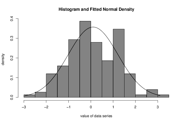
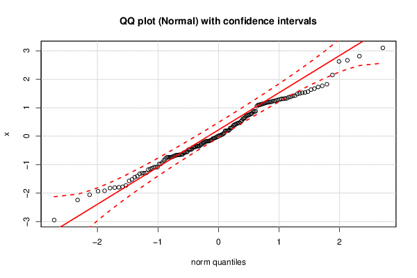
Title produced by software

ML Fitting and QQ Plot- Normal Distribution

Date of computation

Sat, 07 Nov 2015 10:34:26 +0000

Cite this page as follows

Statistical Computations at FreeStatistics.org, Office for Research Development and Education, URL https://freestatistics.org/blog/index.php?v=date/2015/Nov/07/t1446892489ysulph2lumidswm.htm/, Retrieved Tue, 14 May 2024 04:10:47 +0000

Statistical Computations at FreeStatistics.org, Office for Research Development and Education, URL https://freestatistics.org/blog/index.php?pk=283209, Retrieved Tue, 14 May 2024 04:10:47 +0000

QR Codes:

Paste this QR Code to cite your computation.

Original text written by user:

IsPrivate?

No (this computation is public)

User-defined keywords

Estimated Impact

124

Family? (F = Feedback message, R = changed R code, M = changed R Module, P = changed Parameters, D = changed Data)

-       [ML Fitting and QQ Plot- Normal Distribution] [Task 12 - Chapter...] [2015-11-07 10:34:26] [39661ea0cc1af7d66f31b3ef3719ea7a] [Current]

Feedback Forum

Post a new message

Dataseries X:

Download CSV

Histogram

Boxplots

-1.299916663
0.1884719613
0.05838156396
0.5093151731
1.31272113
-0.1304945692
0.3725055164
-0.5499759343
-0.6967597071
1.112034826
1.370482656
-0.1750114035
-0.1752429122
1.156007102
-0.1819366812
-1.288829354
-0.1573992949
1.419335663
-1.917665431
-0.4508939494
-1.931970739
-0.6504155989
-0.9736268635
-0.7944732244
-0.6861797408
0.1975275493
1.325773885
-0.04214209448
-1.728263306
0.7125841242
-1.792946872
0.4005898175
-0.2881321908
-2.239872365
-0.3920731506
1.273525125
1.103844858
-0.1393296612
0.7594643691
1.211900984
0.6599319935
-0.3490766567
1.190116145
-0.5816142599
-0.2000079972
-0.7332693054
2.151617507
1.256951579
0.03832716464
-0.3521209543
0.4667666728
1.768620958
1.292395144
-0.235217552
0.7990784653
0.1090892455
0.6133998414
-0.2329583707
-0.6556878519
-1.091778622
-0.6612430777
-2.94612105
-2.056124843
0.551424181
2.666434937
-0.7335526186
-0.3798989136
1.38289334
-0.3488289378
1.20201579
1.533403298
-0.1692645449
0.6225618849
-0.3499720683
-0.6386968225
0.4539651432
-0.9749707474
-0.8499628341
1.09933319
-1.088622878
-1.320338928
1.671516316
0.2838155993
-1.147706775
0.4679270678
0.2155419059
1.636515492
1.729184585
0.4372698037
-0.6616461585
1.131169198
-0.4678314368
1.328570322
-1.403210056
-1.518112415
-0.5546191141
-0.4745109955
-1.084404369
1.053434578
1.425222765
-0.5743186471
-1.123391654
0.1933801173
-1.299517169
1.233888988
-0.07018270534
-0.01387122401
-1.805665665
-1.823094763
1.526297851
-1.571177073
0.8682072802
1.140416026
1.173021125
0.0291210346
-0.01246486712
0.727715883
0.4095388145
1.824851223
1.309377425
0.7402984735
-0.2934576427
-1.174460657
1.191916363
0.08032260499
0.2862977658
0.8758122862
2.625829103
-0.9250469882
0.8649551389
-0.05932339715
0.1875348972
-1.777423877
0.3167333151
2.812671353
-0.08568303965
-0.639108989
-0.7400207945
1.240896848
3.10131965
-0.7431251116
1.565102671
1.481917808
0.02042061539
-0.3813755101
0.7843858381
-0.7274583899
-1.439022351
-0.4709286982
1.503667829

Summary of computational transaction
Raw Input	view raw input (R code)
Raw Output	view raw output of R engine
Computing time	3 seconds
R Server	'Sir Maurice George Kendall' @ kendall.wessa.net

\begin{tabular}{lllllllll}
\hline
Summary of computational transaction \tabularnewline
Raw Input & view raw input (R code)  \tabularnewline
Raw Output & view raw output of R engine  \tabularnewline
Computing time & 3 seconds \tabularnewline
R Server & 'Sir Maurice George Kendall' @ kendall.wessa.net \tabularnewline
\hline
\end{tabular}
%Source: https://freestatistics.org/blog/index.php?pk=283209&T=0

[TABLE]
[ROW][C]Summary of computational transaction[/C][/ROW]
[ROW][C]Raw Input[/C][C]view raw input (R code) [/C][/ROW]
[ROW][C]Raw Output[/C][C]view raw output of R engine [/C][/ROW]
[ROW][C]Computing time[/C][C]3 seconds[/C][/ROW]
[ROW][C]R Server[/C][C]'Sir Maurice George Kendall' @ kendall.wessa.net[/C][/ROW]
[/TABLE]
Source: https://freestatistics.org/blog/index.php?pk=283209&T=0

Globally Unique Identifier (entire table): ba.freestatistics.org/blog/index.php?pk=283209&T=0

As an alternative you can also use a QR Code:

The GUIDs for individual cells are displayed in the table below:

Summary of computational transaction
Raw Input	view raw input (R code)
Raw Output	view raw output of R engine
Computing time	3 seconds
R Server	'Sir Maurice George Kendall' @ kendall.wessa.net

Parameter	Estimated Value	Standard Deviation
mean	0.1009587778042	0.0912193464321452
standard deviation	1.11720426714462	0.0645018184375747

\begin{tabular}{lllllllll}
\hline
Parameter & Estimated Value & Standard Deviation \tabularnewline
mean & 0.1009587778042 & 0.0912193464321452 \tabularnewline
standard deviation & 1.11720426714462 & 0.0645018184375747 \tabularnewline
\hline
\end{tabular}
%Source: https://freestatistics.org/blog/index.php?pk=283209&T=1

[TABLE]
[ROW][C]Parameter[/C][C]Estimated Value[/C][C]Standard Deviation[/C][/ROW]
[ROW][C]mean[/C][C]0.1009587778042[/C][C]0.0912193464321452[/C][/ROW]
[ROW][C]standard deviation[/C][C]1.11720426714462[/C][C]0.0645018184375747[/C][/ROW]
[/TABLE]
Source: https://freestatistics.org/blog/index.php?pk=283209&T=1

Globally Unique Identifier (entire table): ba.freestatistics.org/blog/index.php?pk=283209&T=1

As an alternative you can also use a QR Code:

The GUIDs for individual cells are displayed in the table below:

Parameter	Estimated Value	Standard Deviation
mean	0.1009587778042	0.0912193464321452
standard deviation	1.11720426714462	0.0645018184375747

Figure 1

PNG link

Postscript link

PDF link

Figure 2

PNG link

Postscript link

PDF link

Parameters (Session):

Parameters (R input):

par1 = 8 ; par2 = 0 ;

R code (references can be found in the software module):

library(MASS)
library(car)
par1 <- as.numeric(par1)
if (par2 == '0') par2 = 'Sturges' else par2 <- as.numeric(par2)
x <- as.ts(x) #otherwise the fitdistr function does not work properly
r <- fitdistr(x,'normal')
r
bitmap(file='test1.png')
myhist<-hist(x,col=par1,breaks=par2,main=main,ylab=ylab,xlab=xlab,freq=F)
curve(1/(r$estimate[2]*sqrt(2*pi))*exp(-1/2*((x-r$estimate[1])/r$estimate[2])^2),min(x),max(x),add=T)
dev.off()
bitmap(file='test3.png')
qqPlot(x,dist='norm',main='QQ plot (Normal) with confidence intervals')
grid()
dev.off()
load(file='createtable')
a<-table.start()
a<-table.row.start(a)
a<-table.element(a,'Parameter',1,TRUE)
a<-table.element(a,'Estimated Value',1,TRUE)
a<-table.element(a,'Standard Deviation',1,TRUE)
a<-table.row.end(a)
a<-table.row.start(a)
a<-table.element(a,'mean',header=TRUE)
a<-table.element(a,r$estimate[1])
a<-table.element(a,r$sd[1])
a<-table.row.end(a)
a<-table.row.start(a)
a<-table.element(a,'standard deviation',header=TRUE)
a<-table.element(a,r$estimate[2])
a<-table.element(a,r$sd[2])
a<-table.row.end(a)
a<-table.end(a)
table.save(a,file='mytable.tab')

Free Statistics

Description of Statistical Computation

Tree of Dependent Computations

Dataset

Tables (Output of Computation)

Figures (Output of Computation)

Input Parameters & R Code