Repository of Reproducible Computations

Free Statistics

of Irreproducible Research!

Author's title

Author

*The author of this computation has been verified*

R Software Module

rwasp_fitdistrchisq1.wasp

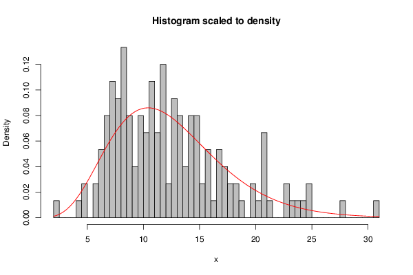
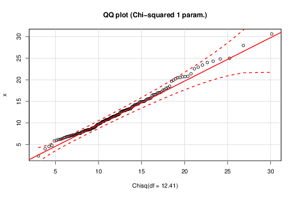
Title produced by software

Maximum-likelihood Fitting - Chi-squared Distribution

Date of computation

Fri, 06 Nov 2015 12:10:59 +0000

Cite this page as follows

Statistical Computations at FreeStatistics.org, Office for Research Development and Education, URL https://freestatistics.org/blog/index.php?v=date/2015/Nov/06/t144681189171d5dap77o69ndi.htm/, Retrieved Mon, 13 May 2024 23:18:51 +0000

Statistical Computations at FreeStatistics.org, Office for Research Development and Education, URL https://freestatistics.org/blog/index.php?pk=283173, Retrieved Mon, 13 May 2024 23:18:51 +0000

QR Codes:

Paste this QR Code to cite your computation.

Original text written by user:

IsPrivate?

No (this computation is public)

User-defined keywords

Estimated Impact

162

Family? (F = Feedback message, R = changed R code, M = changed R Module, P = changed Parameters, D = changed Data)

-       [Maximum-likelihood Fitting - Chi-squared Distribution] [Task 5 - Chapter ...] [2015-11-06 12:10:59] [39661ea0cc1af7d66f31b3ef3719ea7a] [Current]

Feedback Forum

Post a new message

Dataseries X:

Download CSV

Histogram

Boxplots

2.367183298
12.76478264
8.827608601
24.81198807
11.63177126
9.437115101
13.78035738
12.61257426
21.39267951
10.7862099
14.91088905
20.51389771
12.61561577
9.801653014
6.85179221
14.20739816
13.84213921
8.266703576
6.182929006
14.30674421
14.93214147
19.93222303
15.20801523
7.499792454
14.42486076
7.971297014
8.471255733
10.33837883
10.73754186
12.88654485
9.738211508
7.923133712
11.40779047
10.24936017
8.593957689
30.6148155
27.94941976
13.51785308
7.191023993
11.11868007
7.095088307
11.36199654
4.568219985
20.72923664
13.0877668
15.60956273
8.061288934
12.46848507
8.356443382
8.472587207
11.92345777
11.58422641
7.216937154
9.569506477
10.86982316
16.53230418
20.23741381
17.67871686
13.15837305
17.03165732
22.93247777
10.36634471
18.50341727
10.3146623
14.93925202
8.868169698
6.924769981
6.830307971
24.98880039
14.81397449
14.20155811
6.40300417
18.164978
8.876133817
22.54014269
7.621925382
15.69939447
16.93454617
14.36795552
7.905300659
17.00451212
16.55931391
4.018173352
6.292944919
7.450204394
13.24356804
7.214089738
17.61657515
23.40951583
7.585151174
20.82777864
12.93276224
11.86978734
6.156490144
9.142292663
8.191126732
20.55001555
9.883280955
17.2144518
11.30565512
16.5653778
8.783932027
11.91919856
14.99800664
14.96042102
10.95565957
24.29347583
8.405293504
8.957710969
8.48309493
6.61290138
13.28136459
12.85869774
18.06094603
5.857802506
6.940157679
11.18358028
15.57662791
10.53627317
11.70804827
12.22415801
7.265098592
11.57767448
14.02502462
16.3737557
8.246029843
7.592008456
19.69353365
12.77552298
20.70935008
7.149189576
5.981773487
8.399400217
7.58068928
10.61663385
13.10957305
10.0155854
15.41656012
23.98578818
6.645769864
4.795559247
9.935652687
9.689349403
10.72420255
10.83209602
13.26502537
15.78021629
11.51832358
11.99285559
9.21067046

Summary of computational transaction
Raw Input	view raw input (R code)
Raw Output	view raw output of R engine
Computing time	3 seconds
R Server	'George Udny Yule' @ yule.wessa.net

\begin{tabular}{lllllllll}
\hline
Summary of computational transaction \tabularnewline
Raw Input & view raw input (R code)  \tabularnewline
Raw Output & view raw output of R engine  \tabularnewline
Computing time & 3 seconds \tabularnewline
R Server & 'George Udny Yule' @ yule.wessa.net \tabularnewline
\hline
\end{tabular}
%Source: https://freestatistics.org/blog/index.php?pk=283173&T=0

[TABLE]
[ROW][C]Summary of computational transaction[/C][/ROW]
[ROW][C]Raw Input[/C][C]view raw input (R code) [/C][/ROW]
[ROW][C]Raw Output[/C][C]view raw output of R engine [/C][/ROW]
[ROW][C]Computing time[/C][C]3 seconds[/C][/ROW]
[ROW][C]R Server[/C][C]'George Udny Yule' @ yule.wessa.net[/C][/ROW]
[/TABLE]
Source: https://freestatistics.org/blog/index.php?pk=283173&T=0

Globally Unique Identifier (entire table): ba.freestatistics.org/blog/index.php?pk=283173&T=0

As an alternative you can also use a QR Code:

The GUIDs for individual cells are displayed in the table below:

Summary of computational transaction
Raw Input	view raw input (R code)
Raw Output	view raw output of R engine
Computing time	3 seconds
R Server	'George Udny Yule' @ yule.wessa.net

Parameter	Estimated Value	Standard Deviation
df	12.4144525491007	0.390613568455056

\begin{tabular}{lllllllll}
\hline
Parameter & Estimated Value & Standard Deviation \tabularnewline
df & 12.4144525491007 & 0.390613568455056 \tabularnewline
\hline
\end{tabular}
%Source: https://freestatistics.org/blog/index.php?pk=283173&T=1

[TABLE]
[ROW][C]Parameter[/C][C]Estimated Value[/C][C]Standard Deviation[/C][/ROW]
[ROW][C]df[/C][C]12.4144525491007[/C][C]0.390613568455056[/C][/ROW]
[/TABLE]
Source: https://freestatistics.org/blog/index.php?pk=283173&T=1

Globally Unique Identifier (entire table): ba.freestatistics.org/blog/index.php?pk=283173&T=1

As an alternative you can also use a QR Code:

The GUIDs for individual cells are displayed in the table below:

Parameter	Estimated Value	Standard Deviation
df	12.4144525491007	0.390613568455056

Figure 1

PNG link

Postscript link

PDF link

Figure 2

PNG link

Postscript link

PDF link

Parameters (Session):

Parameters (R input):

R code (references can be found in the software module):

library(MASS)
library(car)
chii <- x
chi_df <- fitdistr(chii,'chi-squared',start=list(df=3), method='Brent',lower=0.1,upper=100)
chi_k <- chi_df[[1]][1]
bitmap(file='test1.png')
chi_hist <- hist(chii,breaks=50,col='gray',freq=FALSE,main='Histogram scaled to density',xlab='x')
curve(dchisq(x,df=chi_k),add=TRUE,col='red')
dev.off()
f<-chi_df
f$estimate
f$sd
xlab <- paste('Chisq(df = ',round(f$estimate[[1]],2),sep='')
xlab <- paste(xlab,')',sep='')
xlab
bitmap(file='test2.png')
qqPlot(x, dist='chisq', df=f$estimate[[1]], ncp=0, main='QQ plot (Chi-squared 1 param.)', xlab=xlab )
grid()
dev.off()
load(file='createtable')
a<-table.start()
a<-table.row.start(a)
a<-table.element(a,'Parameter',1,TRUE)
a<-table.element(a,'Estimated Value',1,TRUE)
a<-table.element(a,'Standard Deviation',1,TRUE)
a<-table.row.end(a)
a<-table.row.start(a)
a<-table.element(a,'df',header=TRUE)
a<-table.element(a,f$estimate[1])
a<-table.element(a,f$sd[1])
a<-table.row.end(a)
a<-table.end(a)
table.save(a,file='mytable.tab')

Free Statistics

Description of Statistical Computation

Tree of Dependent Computations

Dataset

Tables (Output of Computation)

Figures (Output of Computation)

Input Parameters & R Code