Free Statistics
of Irreproducible Research!
Description of Statistical Computation | |||||||||||||||||||||||||||||||||||||||
|---|---|---|---|---|---|---|---|---|---|---|---|---|---|---|---|---|---|---|---|---|---|---|---|---|---|---|---|---|---|---|---|---|---|---|---|---|---|---|---|
| Author's title | |||||||||||||||||||||||||||||||||||||||
| Author | *The author of this computation has been verified* | ||||||||||||||||||||||||||||||||||||||
| R Software Module | rwasp_fitdistrnorm.wasp | ||||||||||||||||||||||||||||||||||||||
| Title produced by software | ML Fitting and QQ Plot- Normal Distribution | ||||||||||||||||||||||||||||||||||||||
| Date of computation | Fri, 06 Nov 2015 12:01:20 +0000 | ||||||||||||||||||||||||||||||||||||||
| Cite this page as follows | Statistical Computations at FreeStatistics.org, Office for Research Development and Education, URL https://freestatistics.org/blog/index.php?v=date/2015/Nov/06/t1446811298pcoip2yc5p1z5ue.htm/, Retrieved Mon, 13 May 2024 22:07:33 +0000 | ||||||||||||||||||||||||||||||||||||||
| Statistical Computations at FreeStatistics.org, Office for Research Development and Education, URL https://freestatistics.org/blog/index.php?pk=283169, Retrieved Mon, 13 May 2024 22:07:33 +0000 | |||||||||||||||||||||||||||||||||||||||
| QR Codes: | |||||||||||||||||||||||||||||||||||||||
|
| |||||||||||||||||||||||||||||||||||||||
| Original text written by user: | |||||||||||||||||||||||||||||||||||||||
| IsPrivate? | No (this computation is public) | ||||||||||||||||||||||||||||||||||||||
| User-defined keywords | |||||||||||||||||||||||||||||||||||||||
| Estimated Impact | 160 | ||||||||||||||||||||||||||||||||||||||
Tree of Dependent Computations | |||||||||||||||||||||||||||||||||||||||
| Family? (F = Feedback message, R = changed R code, M = changed R Module, P = changed Parameters, D = changed Data) | |||||||||||||||||||||||||||||||||||||||
| - [ML Fitting and QQ Plot- Normal Distribution] [Task 4 - Chapter 3] [2015-11-06 12:01:20] [39661ea0cc1af7d66f31b3ef3719ea7a] [Current] | |||||||||||||||||||||||||||||||||||||||
| Feedback Forum | |||||||||||||||||||||||||||||||||||||||
Post a new message | |||||||||||||||||||||||||||||||||||||||
Dataset | |||||||||||||||||||||||||||||||||||||||
| Dataseries X: | |||||||||||||||||||||||||||||||||||||||
5.192811936 8.077925175 13.20295159 5.637742324 20.74485033 10.07621753 8.635968458 9.572465177 5.986244204 8.681694758 8.762467616 9.447984369 13.23223239 6.424477277 11.15027122 5.66394648 5.833589471 15.36063712 9.991390024 7.356232709 11.30582961 5.175803061 20.76726409 4.792299852 10.40326875 13.23253865 10.02054783 8.100592711 8.516183524 10.53687311 12.38572858 13.91814131 8.183820276 15.57604046 3.651330699 8.54006787 15.05167067 10.87236063 9.784830049 14.96336567 20.40044109 9.754087505 10.38236058 9.792647428 5.544281539 6.053143837 8.904190524 13.10490619 19.10554882 15.0512861 7.969304159 19.75793495 7.743242759 4.206002829 18.83038299 23.49988057 18.37928404 10.75642957 15.08295323 14.95797357 6.479159716 8.878326303 14.19955706 11.02062257 17.96369791 13.27622938 11.25675776 5.92598552 10.9261522 10.33654365 12.06832183 11.41785376 6.531835283 8.796448015 13.1826687 9.919088022 13.43244363 7.844999913 18.19910412 15.4031689 5.113264518 9.005734297 18.64259048 12.37957064 8.32370786 16.75634285 9.857722644 11.53602073 3.266256321 11.97771886 6.979379364 19.88740278 9.649501137 6.799058625 6.368776666 13.68949125 13.25195424 5.352454016 7.440884757 5.590030277 15.5023281 10.55990617 21.7367648 10.84992249 6.317396275 17.67422845 10.30467645 9.816795137 15.23007634 8.645079123 7.151047018 8.621973543 21.1938828 10.15623273 10.23509062 13.82680211 3.93144154 6.378395723 8.40335876 15.82177585 12.57112898 15.15518719 8.17972718 7.332399891 7.074727383 11.36768646 13.05583415 21.19169274 16.78718574 5.601719977 9.260754771 15.27314003 25.95435851 17.18026098 18.85473086 18.97684559 8.831133132 12.99127941 7.154082925 8.998621136 24.70477524 11.13819866 18.53340344 9.077564335 7.984510263 13.88274951 6.405538375 15.16551006 20.35454414 20.03279111 | |||||||||||||||||||||||||||||||||||||||
Tables (Output of Computation) | |||||||||||||||||||||||||||||||||||||||
| |||||||||||||||||||||||||||||||||||||||
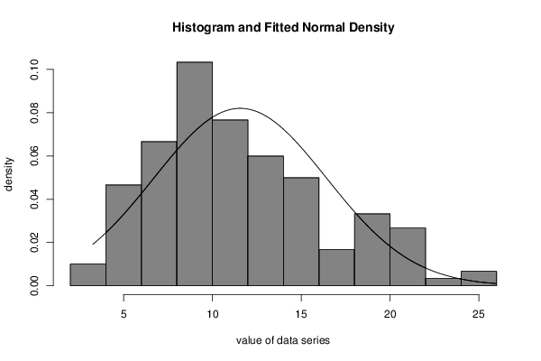
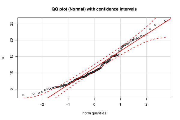
Figures (Output of Computation) | |||||||||||||||||||||||||||||||||||||||
Input Parameters & R Code | |||||||||||||||||||||||||||||||||||||||
| Parameters (Session): | |||||||||||||||||||||||||||||||||||||||
| par1 = 8 ; par2 = 0 ; | |||||||||||||||||||||||||||||||||||||||
| Parameters (R input): | |||||||||||||||||||||||||||||||||||||||
| par1 = 8 ; par2 = 0 ; | |||||||||||||||||||||||||||||||||||||||
| R code (references can be found in the software module): | |||||||||||||||||||||||||||||||||||||||
library(MASS) | |||||||||||||||||||||||||||||||||||||||