Free Statistics
of Irreproducible Research!
Description of Statistical Computation | |||||||||||||||||||||||||||||||||||||||
|---|---|---|---|---|---|---|---|---|---|---|---|---|---|---|---|---|---|---|---|---|---|---|---|---|---|---|---|---|---|---|---|---|---|---|---|---|---|---|---|
| Author's title | |||||||||||||||||||||||||||||||||||||||
| Author | *The author of this computation has been verified* | ||||||||||||||||||||||||||||||||||||||
| R Software Module | rwasp_fitdistrnorm.wasp | ||||||||||||||||||||||||||||||||||||||
| Title produced by software | ML Fitting and QQ Plot- Normal Distribution | ||||||||||||||||||||||||||||||||||||||
| Date of computation | Fri, 06 Nov 2015 11:57:47 +0000 | ||||||||||||||||||||||||||||||||||||||
| Cite this page as follows | Statistical Computations at FreeStatistics.org, Office for Research Development and Education, URL https://freestatistics.org/blog/index.php?v=date/2015/Nov/06/t1446811084s6avwxhg9g1qem6.htm/, Retrieved Tue, 14 May 2024 01:53:08 +0000 | ||||||||||||||||||||||||||||||||||||||
| Statistical Computations at FreeStatistics.org, Office for Research Development and Education, URL https://freestatistics.org/blog/index.php?pk=283168, Retrieved Tue, 14 May 2024 01:53:08 +0000 | |||||||||||||||||||||||||||||||||||||||
| QR Codes: | |||||||||||||||||||||||||||||||||||||||
|
| |||||||||||||||||||||||||||||||||||||||
| Original text written by user: | |||||||||||||||||||||||||||||||||||||||
| IsPrivate? | No (this computation is public) | ||||||||||||||||||||||||||||||||||||||
| User-defined keywords | |||||||||||||||||||||||||||||||||||||||
| Estimated Impact | 188 | ||||||||||||||||||||||||||||||||||||||
Tree of Dependent Computations | |||||||||||||||||||||||||||||||||||||||
| Family? (F = Feedback message, R = changed R code, M = changed R Module, P = changed Parameters, D = changed Data) | |||||||||||||||||||||||||||||||||||||||
| - [ML Fitting and QQ Plot- Normal Distribution] [Task 3 - Chapter 3] [2015-11-06 11:57:47] [39661ea0cc1af7d66f31b3ef3719ea7a] [Current] | |||||||||||||||||||||||||||||||||||||||
| Feedback Forum | |||||||||||||||||||||||||||||||||||||||
Post a new message | |||||||||||||||||||||||||||||||||||||||
Dataset | |||||||||||||||||||||||||||||||||||||||
| Dataseries X: | |||||||||||||||||||||||||||||||||||||||
3.144526987 -0.06001685076 -0.4001231611 -0.2102028967 -1.501877712 0.2539317116 0.4319650657 0.2775640954 -0.6725003436 0.07055596888 -0.01528606856 0.5057418843 -0.9750275179 0.6820133085 1.511106635 0.4178220937 0.5057376987 0.4407287653 0.8334573132 0.03862111098 -0.6875100621 -0.06177250389 -1.278536709 2.176550196 -0.2330892833 -0.2691565903 0.3171313733 0.6727613303 0.1680326246 0.6123016741 -0.3934201518 0.1971677445 0.0374788857 0.4331769931 1.938715378 -1.408661197 -1.588422733 -0.5327732432 0.5907843312 -0.2417284493 0.1803497339 0.3245985615 1.380799905 -0.9009647023 0.4733761657 0.4119137214 0.3268438613 0.4962925912 0.09253414959 -0.06077516358 0.3532430254 -1.155305405 0.991612865 1.473849233 -0.9563787348 -0.871848343 -2.197197435 -0.9589232286 -0.5591736647 -1.956021227 0.4100587655 0.7717526678 -1.106268722 -0.8260839523 -1.430658558 0.09673579433 0.9509115548 1.702024388 -1.424270625 0.488231622 -0.6988034315 0.6794556835 -0.02259062063 0.7479999909 -1.23890344 0.8360987262 -0.663459618 -0.157561439 -0.6908957299 -0.0609006182 0.03699315031 0.2845403773 1.166871686 1.69825612 1.138964012 -0.9372728844 0.9272619168 -0.7817091942 0.2804644697 0.1165570981 -0.2707241124 -1.002006024 -0.3743147346 1.359308124 1.479854064 -0.5237546484 -1.139764209 1.247435759 -0.8774467744 1.124909402 -1.766741831 -0.1030939538 -1.046901776 -0.911394186 0.6464166683 -0.2535962721 -1.018191091 0.3713550451 -0.2102380471 0.767415034 1.342901398 -0.4299011888 -1.675529831 -0.7788139624 0.7506655097 1.155095643 2.112457454 -0.03744462346 0.002515890948 -0.7028087591 0.4928690114 0.2906622073 0.5289194085 0.2419641872 -0.3945567373 0.3465295564 0.9901961729 -2.769253757 -0.2392484301 0.05752196494 0.9201969647 -0.03148187918 -1.142688072 -0.3713212468 -0.5831455147 -2.36132036 0.8455786891 -0.4190781375 -0.1203894082 1.464695634 0.2388063778 0.3361388849 -1.206282329 -0.1813839503 0.6707893748 -0.6508587643 -0.4385846291 0.8764718594 -1.4995241 -1.213503097 | |||||||||||||||||||||||||||||||||||||||
Tables (Output of Computation) | |||||||||||||||||||||||||||||||||||||||
| |||||||||||||||||||||||||||||||||||||||
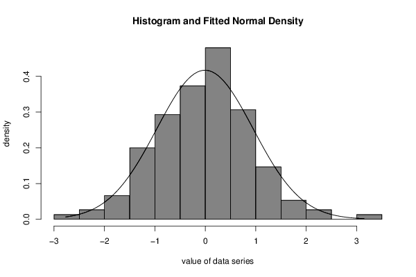
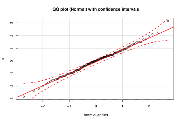
Figures (Output of Computation) | |||||||||||||||||||||||||||||||||||||||
Input Parameters & R Code | |||||||||||||||||||||||||||||||||||||||
| Parameters (Session): | |||||||||||||||||||||||||||||||||||||||
| par1 = 8 ; par2 = 0 ; | |||||||||||||||||||||||||||||||||||||||
| Parameters (R input): | |||||||||||||||||||||||||||||||||||||||
| par1 = 8 ; par2 = 0 ; | |||||||||||||||||||||||||||||||||||||||
| R code (references can be found in the software module): | |||||||||||||||||||||||||||||||||||||||
library(MASS) | |||||||||||||||||||||||||||||||||||||||