Free Statistics
of Irreproducible Research!
Description of Statistical Computation | |||||||||||||||||||||||||||||||||
|---|---|---|---|---|---|---|---|---|---|---|---|---|---|---|---|---|---|---|---|---|---|---|---|---|---|---|---|---|---|---|---|---|---|
| Author's title | |||||||||||||||||||||||||||||||||
| Author | *The author of this computation has been verified* | ||||||||||||||||||||||||||||||||
| R Software Module | rwasp_fitdistrchisq1.wasp | ||||||||||||||||||||||||||||||||
| Title produced by software | Maximum-likelihood Fitting - Chi-squared Distribution | ||||||||||||||||||||||||||||||||
| Date of computation | Wed, 04 Nov 2015 12:44:49 +0000 | ||||||||||||||||||||||||||||||||
| Cite this page as follows | Statistical Computations at FreeStatistics.org, Office for Research Development and Education, URL https://freestatistics.org/blog/index.php?v=date/2015/Nov/04/t14466411206v6veqz3uzbfjsl.htm/, Retrieved Tue, 14 May 2024 23:08:53 +0000 | ||||||||||||||||||||||||||||||||
| Statistical Computations at FreeStatistics.org, Office for Research Development and Education, URL https://freestatistics.org/blog/index.php?pk=283147, Retrieved Tue, 14 May 2024 23:08:53 +0000 | |||||||||||||||||||||||||||||||||
| QR Codes: | |||||||||||||||||||||||||||||||||
|
| |||||||||||||||||||||||||||||||||
| Original text written by user: | |||||||||||||||||||||||||||||||||
| IsPrivate? | No (this computation is public) | ||||||||||||||||||||||||||||||||
| User-defined keywords | |||||||||||||||||||||||||||||||||
| Estimated Impact | 143 | ||||||||||||||||||||||||||||||||
Tree of Dependent Computations | |||||||||||||||||||||||||||||||||
| Family? (F = Feedback message, R = changed R code, M = changed R Module, P = changed Parameters, D = changed Data) | |||||||||||||||||||||||||||||||||
| - [Maximum-likelihood Fitting - Chi-squared Distribution] [3.1. task 5 O] [2015-11-04 12:44:49] [7b81fac622814275349f5d25cf6bd6bd] [Current] | |||||||||||||||||||||||||||||||||
| Feedback Forum | |||||||||||||||||||||||||||||||||
Post a new message | |||||||||||||||||||||||||||||||||
Dataset | |||||||||||||||||||||||||||||||||
| Dataseries X: | |||||||||||||||||||||||||||||||||
11.52220501 13.58673798 16.52179164 11.75787553 15.26558154 13.53792284 12.11256732 11.30045294 9.677625076 14.54512011 6.934478378 12.54042708 5.351628021 4.645078514 6.030218685 15.18962166 5.696765843 10.36002577 11.9530765 5.188436433 7.859623831 12.50231771 7.314319746 17.68569457 22.22053339 4.520819837 8.62219385 11.50023699 9.640562651 14.92425779 11.29702253 15.73543703 8.029408184 8.874105422 20.67956869 9.267024923 12.33611991 7.37538945 10.790783 18.7392901 7.278318046 5.56708414 13.76696924 8.096487687 13.4270164 11.43990029 13.83121614 6.78100946 10.41658736 15.70571604 9.049884866 17.70436149 9.441011579 9.798079662 13.53723312 18.26920705 9.318549528 12.4270619 12.85658507 10.34861522 10.92903052 12.6369996 12.36829015 21.61185646 15.56424122 6.520804808 12.99141728 13.79092895 4.171968283 7.675841074 18.741056 6.837973156 14.33547067 7.675785185 8.01200137 4.311373039 8.309566026 10.20010014 6.828260307 8.588016581 11.64556952 7.675734356 17.28523474 12.66077139 12.08646096 9.321115733 6.629360763 12.42337295 7.228246871 9.174168883 15.52280274 7.266352654 11.86353824 5.998127662 9.100006553 8.172118377 8.872517769 12.55082305 8.324573969 7.430859814 9.649398319 6.058616033 6.828285075 17.76031706 12.34675734 10.15724549 13.43912442 17.25580992 8.243436903 14.3551501 12.5993967 11.32802256 9.321051767 11.46903551 8.505520344 5.813274525 16.66217211 10.03030643 14.00678235 3.943997282 9.02519593 11.74340882 14.47284098 12.97670121 8.112883361 12.91527961 9.501760913 10.99886438 16.74570814 11.90621919 9.849743634 12.74252017 12.1746156 15.36003449 9.660893575 7.659179952 21.75978807 7.949595442 16.79913818 10.06232549 13.9960018 16.55406677 18.00620693 6.700604195 9.747479995 17.41406005 11.22865536 13.07141212 6.274579135 11.81505406 | |||||||||||||||||||||||||||||||||
Tables (Output of Computation) | |||||||||||||||||||||||||||||||||
| |||||||||||||||||||||||||||||||||
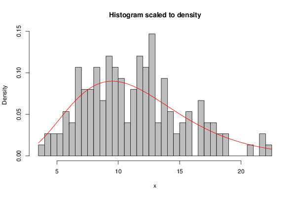
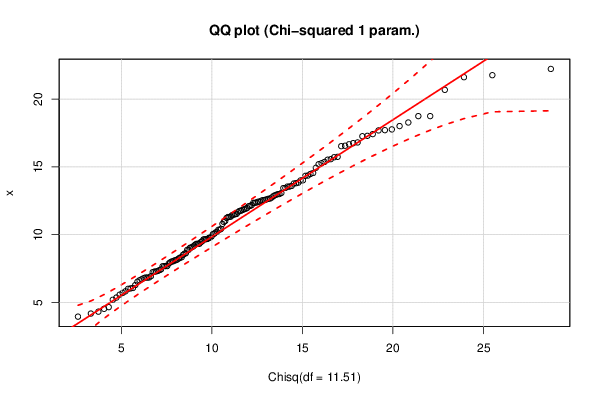
Figures (Output of Computation) | |||||||||||||||||||||||||||||||||
Input Parameters & R Code | |||||||||||||||||||||||||||||||||
| Parameters (Session): | |||||||||||||||||||||||||||||||||
| Parameters (R input): | |||||||||||||||||||||||||||||||||
| R code (references can be found in the software module): | |||||||||||||||||||||||||||||||||
library(MASS) | |||||||||||||||||||||||||||||||||