Repository of Reproducible Computations

Free Statistics

of Irreproducible Research!

Author's title

Author

*The author of this computation has been verified*

R Software Module

rwasp_fitdistrchisq1.wasp

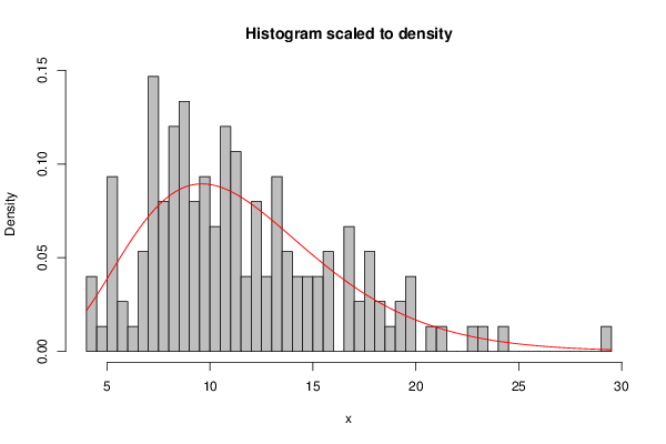
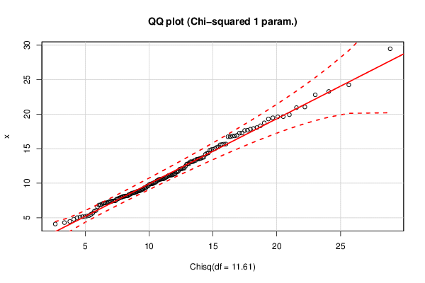
Title produced by software

Maximum-likelihood Fitting - Chi-squared Distribution

Date of computation

Wed, 04 Nov 2015 12:43:49 +0000

Cite this page as follows

Statistical Computations at FreeStatistics.org, Office for Research Development and Education, URL https://freestatistics.org/blog/index.php?v=date/2015/Nov/04/t1446641049ad0cd1l60sgi8c3.htm/, Retrieved Tue, 14 May 2024 22:09:47 +0000

Statistical Computations at FreeStatistics.org, Office for Research Development and Education, URL https://freestatistics.org/blog/index.php?pk=283146, Retrieved Tue, 14 May 2024 22:09:47 +0000

QR Codes:

Paste this QR Code to cite your computation.

Original text written by user:

IsPrivate?

No (this computation is public)

User-defined keywords

Estimated Impact

154

Family? (F = Feedback message, R = changed R code, M = changed R Module, P = changed Parameters, D = changed Data)

-       [Maximum-likelihood Fitting - Chi-squared Distribution] [3.1. task 5] [2015-11-04 12:43:49] [7b81fac622814275349f5d25cf6bd6bd] [Current]

Feedback Forum

Post a new message

Dataseries X:

Download CSV

Histogram

Boxplots

15.56454772
8.876949456
7.343958118
7.363175805
6.985836275
17.63890926
10.61318131
6.58940159
10.64905069
5.477730919
7.970916294
4.462110249
15.60877656
12.75364041
16.85360223
11.02913162
10.84433102
21.03870731
14.79220224
13.60811452
7.14185006
4.293946292
7.855844509
11.12430149
8.569834145
16.73340558
17.92528405
19.61536487
19.92221478
8.37318909
8.606277008
13.29507975
6.840753119
8.887607123
16.74156774
18.06399536
7.699239985
10.53555947
8.115426594
11.1861451
5.656074019
9.814925536
7.948548923
15.65783948
19.3007408
13.2710996
12.82912465
7.43940357
15.00906417
12.08318851
17.26678566
13.54966393
7.38104098
6.854756671
19.47524652
5.252202771
8.645110003
7.123103707
11.33210692
13.47443826
10.92967058
15.67276142
18.74287917
15.26175915
9.578133295
10.16145061
12.16829556
9.163677789
19.64604273
5.007395428
7.445006581
9.94098223
13.1082095
8.099560152
14.87753013
5.145071802
11.24412306
29.47200757
12.17836569
15.17054579
8.446791325
9.130200202
9.902868506
14.31404032
7.085276633
24.24596625
9.59425123
5.098996926
23.28434022
10.63268294
6.051916989
5.149401835
9.021472502
13.49209873
8.361467248
5.956543711
17.82635289
8.152943398
11.38665016
9.873959346
8.159941805
8.729402037
8.071088613
11.14446759
22.80768059
8.725306646
13.1060958
7.192094652
13.11004328
8.580297685
10.38561094
14.16564961
16.92700203
8.862390572
9.337098599
8.991512314
18.3206674
12.82442005
9.93115014
11.18520052
11.65099333
7.442565626
10.55441223
11.76995226
12.01725925
13.76360248
9.388915157
7.696450456
11.63307348
5.299409587
12.07562221
10.36378527
7.806121105
10.10132553
17.25161027
10.74723524
14.39036882
17.66819629
7.256418974
10.07709178
4.776487071
12.46711669
14.89777528
9.359603617
16.82826914
20.94596906
4.087225365
10.56653729
13.71257317
8.179088244

Summary of computational transaction
Raw Input	view raw input (R code)
Raw Output	view raw output of R engine
Computing time	4 seconds
R Server	'Sir Ronald Aylmer Fisher' @ fisher.wessa.net

\begin{tabular}{lllllllll}
\hline
Summary of computational transaction \tabularnewline
Raw Input & view raw input (R code)  \tabularnewline
Raw Output & view raw output of R engine  \tabularnewline
Computing time & 4 seconds \tabularnewline
R Server & 'Sir Ronald Aylmer Fisher' @ fisher.wessa.net \tabularnewline
\hline
\end{tabular}
%Source: https://freestatistics.org/blog/index.php?pk=283146&T=0

[TABLE]
[ROW][C]Summary of computational transaction[/C][/ROW]
[ROW][C]Raw Input[/C][C]view raw input (R code) [/C][/ROW]
[ROW][C]Raw Output[/C][C]view raw output of R engine [/C][/ROW]
[ROW][C]Computing time[/C][C]4 seconds[/C][/ROW]
[ROW][C]R Server[/C][C]'Sir Ronald Aylmer Fisher' @ fisher.wessa.net[/C][/ROW]
[/TABLE]
Source: https://freestatistics.org/blog/index.php?pk=283146&T=0

Globally Unique Identifier (entire table): ba.freestatistics.org/blog/index.php?pk=283146&T=0

As an alternative you can also use a QR Code:

The GUIDs for individual cells are displayed in the table below:

Summary of computational transaction
Raw Input	view raw input (R code)
Raw Output	view raw output of R engine
Computing time	4 seconds
R Server	'Sir Ronald Aylmer Fisher' @ fisher.wessa.net

Parameter	Estimated Value	Standard Deviation
df	11.6129423946624	0.376723798266326

\begin{tabular}{lllllllll}
\hline
Parameter & Estimated Value & Standard Deviation \tabularnewline
df & 11.6129423946624 & 0.376723798266326 \tabularnewline
\hline
\end{tabular}
%Source: https://freestatistics.org/blog/index.php?pk=283146&T=1

[TABLE]
[ROW][C]Parameter[/C][C]Estimated Value[/C][C]Standard Deviation[/C][/ROW]
[ROW][C]df[/C][C]11.6129423946624[/C][C]0.376723798266326[/C][/ROW]
[/TABLE]
Source: https://freestatistics.org/blog/index.php?pk=283146&T=1

Globally Unique Identifier (entire table): ba.freestatistics.org/blog/index.php?pk=283146&T=1

As an alternative you can also use a QR Code:

The GUIDs for individual cells are displayed in the table below:

Parameter	Estimated Value	Standard Deviation
df	11.6129423946624	0.376723798266326

Figure 1

PNG link

Postscript link

PDF link

Figure 2

PNG link

Postscript link

PDF link

Parameters (Session):

Parameters (R input):

R code (references can be found in the software module):

library(MASS)
library(car)
chii <- x
chi_df <- fitdistr(chii,'chi-squared',start=list(df=3), method='Brent',lower=0.1,upper=100)
chi_k <- chi_df[[1]][1]
bitmap(file='test1.png')
chi_hist <- hist(chii,breaks=50,col='gray',freq=FALSE,main='Histogram scaled to density',xlab='x')
curve(dchisq(x,df=chi_k),add=TRUE,col='red')
dev.off()
f<-chi_df
f$estimate
f$sd
xlab <- paste('Chisq(df = ',round(f$estimate[[1]],2),sep='')
xlab <- paste(xlab,')',sep='')
xlab
bitmap(file='test2.png')
qqPlot(x, dist='chisq', df=f$estimate[[1]], ncp=0, main='QQ plot (Chi-squared 1 param.)', xlab=xlab )
grid()
dev.off()
load(file='createtable')
a<-table.start()
a<-table.row.start(a)
a<-table.element(a,'Parameter',1,TRUE)
a<-table.element(a,'Estimated Value',1,TRUE)
a<-table.element(a,'Standard Deviation',1,TRUE)
a<-table.row.end(a)
a<-table.row.start(a)
a<-table.element(a,'df',header=TRUE)
a<-table.element(a,f$estimate[1])
a<-table.element(a,f$sd[1])
a<-table.row.end(a)
a<-table.end(a)
table.save(a,file='mytable.tab')

Free Statistics

Description of Statistical Computation

Tree of Dependent Computations

Dataset

Tables (Output of Computation)

Figures (Output of Computation)

Input Parameters & R Code