Repository of Reproducible Computations

Free Statistics

of Irreproducible Research!

Author's title

Author

*The author of this computation has been verified*

R Software Module

rwasp_fitdistrchisq1.wasp

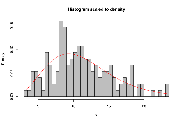
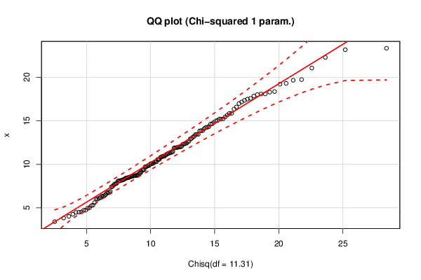
Title produced by software

Maximum-likelihood Fitting - Chi-squared Distribution

Date of computation

Mon, 02 Nov 2015 20:55:16 +0000

Cite this page as follows

Statistical Computations at FreeStatistics.org, Office for Research Development and Education, URL https://freestatistics.org/blog/index.php?v=date/2015/Nov/02/t1446497742agvvu97k26tqm6r.htm/, Retrieved Tue, 14 May 2024 11:36:44 +0000

Statistical Computations at FreeStatistics.org, Office for Research Development and Education, URL https://freestatistics.org/blog/index.php?pk=283125, Retrieved Tue, 14 May 2024 11:36:44 +0000

QR Codes:

Paste this QR Code to cite your computation.

Original text written by user:

IsPrivate?

No (this computation is public)

User-defined keywords

Estimated Impact

162

Family? (F = Feedback message, R = changed R code, M = changed R Module, P = changed Parameters, D = changed Data)

-       [Maximum-likelihood Fitting - Chi-squared Distribution] [Problems Chapter ...] [2015-11-02 20:55:16] [056331f8739198d7705ae45a22f1e54e] [Current]

Feedback Forum

Post a new message

Dataseries X:

Download CSV

Histogram

Boxplots

11.99336739
11.33864658
21.06448093
4.953270113
10.30554294
22.29183208
13.45128912
11.22125691
13.87182042
10.57817899
13.23148907
9.706514628
9.847930133
11.97446486
8.489401722
9.972688199
10.93323793
10.91633214
8.53744425
9.388544504
11.9031245
11.39540062
8.721917071
18.29587148
15.87124909
17.85808921
6.392070818
8.234019423
19.66218291
4.528593135
8.193390044
8.483413475
17.35661629
6.734033041
10.08536924
8.106581064
13.87231369
7.768427825
15.65802797
7.483714049
9.006525779
8.10253392
17.48864642
8.138485814
8.751691905
7.407454625
19.21258807
14.09904698
15.03469408
11.87149051
8.671565018
11.06513676
9.387377946
9.170810741
6.806316534
16.35954272
4.713728444
4.737428987
6.336365506
18.08872955
14.22610309
6.026476369
14.3240286
6.707910545
13.45400458
12.56834133
13.84672281
15.85261421
11.31955921
5.24167967
6.170409225
8.639572449
12.00335878
10.92175284
5.598700084
5.317250182
9.327577247
8.617170722
10.56628874
14.61336289
12.43469518
10.27677494
18.36800852
18.0935586
9.853501613
8.97258727
12.0854163
11.45819407
13.42912584
12.39478677
6.09354129
19.30613092
12.97589044
12.67703025
11.1327705
8.08283201
8.262464764
10.78610615
10.10174275
18.01182554
10.07181674
9.723434465
10.55324035
12.3146117
8.427542832
4.483799895
8.431955611
16.58925427
8.717432347
3.833925275
6.892759742
19.7392398
8.660027879
7.614375499
4.49766246
4.017174647
11.90311074
14.65852426
6.014005932
7.745711907
8.368976509
17.58500475
8.825891553
6.512861937
8.699351084
4.261863088
10.29794782
14.99109735
6.325583274
14.25779314
15.45442704
11.24910346
23.34138897
7.85420562
12.3371357
10.14431909
15.20769125
11.93833677
5.026072809
16.99452582
3.412874049
15.19493846
23.17441517
9.78499816
15.19654434
17.16481748
14.81910776
13.13091197
10.86285191
12.92769388

Summary of computational transaction
Raw Input	view raw input (R code)
Raw Output	view raw output of R engine
Computing time	4 seconds
R Server	'Gwilym Jenkins' @ jenkins.wessa.net

\begin{tabular}{lllllllll}
\hline
Summary of computational transaction \tabularnewline
Raw Input & view raw input (R code)  \tabularnewline
Raw Output & view raw output of R engine  \tabularnewline
Computing time & 4 seconds \tabularnewline
R Server & 'Gwilym Jenkins' @ jenkins.wessa.net \tabularnewline
\hline
\end{tabular}
%Source: https://freestatistics.org/blog/index.php?pk=283125&T=0

[TABLE]
[ROW][C]Summary of computational transaction[/C][/ROW]
[ROW][C]Raw Input[/C][C]view raw input (R code) [/C][/ROW]
[ROW][C]Raw Output[/C][C]view raw output of R engine [/C][/ROW]
[ROW][C]Computing time[/C][C]4 seconds[/C][/ROW]
[ROW][C]R Server[/C][C]'Gwilym Jenkins' @ jenkins.wessa.net[/C][/ROW]
[/TABLE]
Source: https://freestatistics.org/blog/index.php?pk=283125&T=0

Globally Unique Identifier (entire table): ba.freestatistics.org/blog/index.php?pk=283125&T=0

As an alternative you can also use a QR Code:

The GUIDs for individual cells are displayed in the table below:

Summary of computational transaction
Raw Input	view raw input (R code)
Raw Output	view raw output of R engine
Computing time	4 seconds
R Server	'Gwilym Jenkins' @ jenkins.wessa.net

Parameter	Estimated Value	Standard Deviation
df	11.3114215568377	0.37136565066896

\begin{tabular}{lllllllll}
\hline
Parameter & Estimated Value & Standard Deviation \tabularnewline
df & 11.3114215568377 & 0.37136565066896 \tabularnewline
\hline
\end{tabular}
%Source: https://freestatistics.org/blog/index.php?pk=283125&T=1

[TABLE]
[ROW][C]Parameter[/C][C]Estimated Value[/C][C]Standard Deviation[/C][/ROW]
[ROW][C]df[/C][C]11.3114215568377[/C][C]0.37136565066896[/C][/ROW]
[/TABLE]
Source: https://freestatistics.org/blog/index.php?pk=283125&T=1

Globally Unique Identifier (entire table): ba.freestatistics.org/blog/index.php?pk=283125&T=1

As an alternative you can also use a QR Code:

The GUIDs for individual cells are displayed in the table below:

Parameter	Estimated Value	Standard Deviation
df	11.3114215568377	0.37136565066896

Figure 1

PNG link

Postscript link

PDF link

Figure 2

PNG link

Postscript link

PDF link

Parameters (Session):

Parameters (R input):

R code (references can be found in the software module):

library(MASS)
library(car)
chii <- x
chi_df <- fitdistr(chii,'chi-squared',start=list(df=3), method='Brent',lower=0.1,upper=100)
chi_k <- chi_df[[1]][1]
bitmap(file='test1.png')
chi_hist <- hist(chii,breaks=50,col='gray',freq=FALSE,main='Histogram scaled to density',xlab='x')
curve(dchisq(x,df=chi_k),add=TRUE,col='red')
dev.off()
f<-chi_df
f$estimate
f$sd
xlab <- paste('Chisq(df = ',round(f$estimate[[1]],2),sep='')
xlab <- paste(xlab,')',sep='')
xlab
bitmap(file='test2.png')
qqPlot(x, dist='chisq', df=f$estimate[[1]], ncp=0, main='QQ plot (Chi-squared 1 param.)', xlab=xlab )
grid()
dev.off()
load(file='createtable')
a<-table.start()
a<-table.row.start(a)
a<-table.element(a,'Parameter',1,TRUE)
a<-table.element(a,'Estimated Value',1,TRUE)
a<-table.element(a,'Standard Deviation',1,TRUE)
a<-table.row.end(a)
a<-table.row.start(a)
a<-table.element(a,'df',header=TRUE)
a<-table.element(a,f$estimate[1])
a<-table.element(a,f$sd[1])
a<-table.row.end(a)
a<-table.end(a)
table.save(a,file='mytable.tab')

Free Statistics

Description of Statistical Computation

Tree of Dependent Computations

Dataset

Tables (Output of Computation)

Figures (Output of Computation)

Input Parameters & R Code