Free Statistics
of Irreproducible Research!
Description of Statistical Computation | |||||||||||||||||||||
|---|---|---|---|---|---|---|---|---|---|---|---|---|---|---|---|---|---|---|---|---|---|
| Author's title | |||||||||||||||||||||
| Author | *Unverified author* | ||||||||||||||||||||
| R Software Module | rwasp_meanplot.wasp | ||||||||||||||||||||
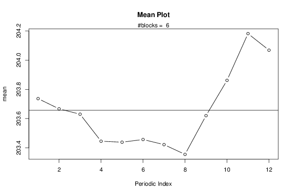
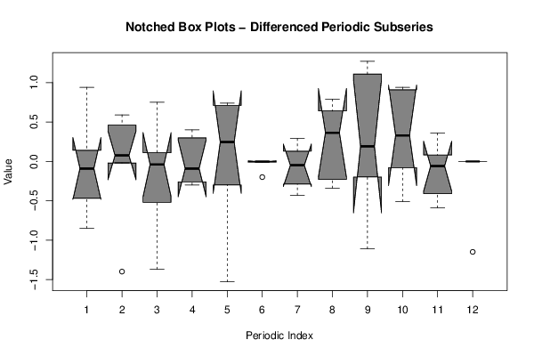
| Title produced by software | Mean Plot | ||||||||||||||||||||
| Date of computation | Sat, 11 Oct 2014 10:42:28 +0100 | ||||||||||||||||||||
| Cite this page as follows | Statistical Computations at FreeStatistics.org, Office for Research Development and Education, URL https://freestatistics.org/blog/index.php?v=date/2014/Oct/11/t1413020638mz7wdgqkfx93k8w.htm/, Retrieved Tue, 14 May 2024 13:40:31 +0000 | ||||||||||||||||||||
| Statistical Computations at FreeStatistics.org, Office for Research Development and Education, URL https://freestatistics.org/blog/index.php?pk=240376, Retrieved Tue, 14 May 2024 13:40:31 +0000 | |||||||||||||||||||||
| QR Codes: | |||||||||||||||||||||
|
| |||||||||||||||||||||
| Original text written by user: | |||||||||||||||||||||
| IsPrivate? | No (this computation is public) | ||||||||||||||||||||
| User-defined keywords | |||||||||||||||||||||
| Estimated Impact | 118 | ||||||||||||||||||||
Tree of Dependent Computations | |||||||||||||||||||||
| Family? (F = Feedback message, R = changed R code, M = changed R Module, P = changed Parameters, D = changed Data) | |||||||||||||||||||||
| - [Mean Plot] [] [2014-10-11 09:42:28] [bdd4dd5e616b71837cf1c04213e8fe07] [Current] | |||||||||||||||||||||
| Feedback Forum | |||||||||||||||||||||
Post a new message | |||||||||||||||||||||
Dataset | |||||||||||||||||||||
| Dataseries X: | |||||||||||||||||||||
204,12 203,27 203,73 203,7 203,44 203,34 203,34 203,05 202,71 202,51 203,45 203,04 203,04 202,87 202,92 202,87 203,17 203,88 203,88 203,45 203,22 202,11 202,5 202,86 202,86 203,8 203,78 204,53 204,44 204,14 204,14 204,04 204,68 205,01 204,93 204,34 204,34 203,87 202,47 201,95 201,86 200,33 200,33 200,33 200,75 201,86 202,77 202,85 202,85 202,84 202,94 203,05 203,45 204,19 204,18 204,47 204,78 206,05 206,32 206,36 205,21 205,35 205,94 204,57 204,27 204,86 204,66 204,79 205,58 205,63 205,12 204,96 | |||||||||||||||||||||
Tables (Output of Computation) | |||||||||||||||||||||
| |||||||||||||||||||||
Figures (Output of Computation) | |||||||||||||||||||||
Input Parameters & R Code | |||||||||||||||||||||
| Parameters (Session): | |||||||||||||||||||||
| par1 = 12 ; | |||||||||||||||||||||
| Parameters (R input): | |||||||||||||||||||||
| par1 = 12 ; | |||||||||||||||||||||
| R code (references can be found in the software module): | |||||||||||||||||||||
par1 <- as.numeric(par1) | |||||||||||||||||||||