Free Statistics

of Irreproducible Research!

Author's title

Author*The author of this computation has been verified*
R Software Modulerwasp_bootstrapplot1.wasp
Title produced by softwareBootstrap Plot - Central Tendency
Date of computationWed, 12 Nov 2014 14:16:29 +0000
Cite this page as followsStatistical Computations at FreeStatistics.org, Office for Research Development and Education, URL https://freestatistics.org/blog/index.php?v=date/2014/Nov/12/t1415802980xksdx2tviegkkjq.htm/, Retrieved Mon, 20 May 2024 01:11:57 +0000
Statistical Computations at FreeStatistics.org, Office for Research Development and Education, URL https://freestatistics.org/blog/index.php?pk=253880, Retrieved Mon, 20 May 2024 01:11:57 +0000
QR Codes:

Original text written by user:
IsPrivate?No (this computation is public)
User-defined keywords
Estimated Impact77
Family? (F = Feedback message, R = changed R code, M = changed R Module, P = changed Parameters, D = changed Data)
-     [Multiple Regression] [WS 7] [2014-11-11 13:27:24] [7b9119a46b6eb1a22eecca7bc054a6e2]
- RMPD    [Bootstrap Plot - Central Tendency] [WS 7 2] [2014-11-12 14:16:29] [a0dc8dfb1ad11084a66a61bab0a3c2c7] [Current]
Feedback Forum

Post a new message
Dataseries X:
587.107
439.575
-549.414
-381.501
-115.339
225.334
417.674
-0.861344
144.883
0.295028
366.746
0.793521
317.516
257.091
-303.976
-214.566
190.899
0.291084
205.985
-230.806
-293.477
-25.819
200.106
0.556907
386.435
704.911
0.424524
-219.186
-155.945
0.150514
-165.134
-628.378
333.677
-188.151
118.054
-0.316327
-32.433
210.987
-533.254
0.322942
24.952
0.0307379
276.711
107.139
572.397
376.932
22.647
-169.324
-0.508219
459.864
-401.529
-109.532
-0.904304
-183.671
-0.614479
261.278
403.091
-588.996
188.311
0.0715541
-170.401
326.829
-0.6281
-360.997
0.101584
-0.682594
0.702586
-314.621
346.557
-0.881513
398.434
-475.978
-293.599
0.402975
158.191
492.103
109.816
0.121907
-489.444
458.191
-2.551
-0.629787
-0.881513
269.608
-269.324
-109.515
171.297
-181.084
-507.068
-0.591763
-378.442
200.847
-220.358
-0.493082
-340.567
309.401
215.484
0.766912
195.178
-315.755
256.661
187.897
-0.885471
-0.39363
-368.048
724.981
236.573
445.746
103.723
651.051
-488.996
-296.707
-551.791
-161.428
293.541
216.056
-298.668
-267.635
-127.531
252.813
-177.809
-135.929
246.143
106.384
-0.425825
-298.739
46.716
682.661
-294.665
164.125
-267.706
-388.415
356.675
-53.672
145.729
-0.981855
-201.709
-0.944628
-350.655
0.896931
-179.876
-34.417
-504.824
-506.221
-0.392221
747.867
-118.686
176.949
-166.103
183.601
26.966
674.934
-270.496
-213.276
0.702388
0.716052
200.847
-362.601
-294.665
-0.208609
-21.962
-0.940501


Summary of computational transaction
Raw Inputview raw input (R code)
Raw Outputview raw output of R engine
Computing time9 seconds
R Server'Sir Maurice George Kendall' @ kendall.wessa.net

\begin{tabular}{lllllllll}
\hline
Summary of computational transaction \tabularnewline
Raw Input & view raw input (R code)  \tabularnewline
Raw Output & view raw output of R engine  \tabularnewline
Computing time & 9 seconds \tabularnewline
R Server & 'Sir Maurice George Kendall' @ kendall.wessa.net \tabularnewline
\hline
\end{tabular}
%Source: https://freestatistics.org/blog/index.php?pk=253880&T=0

[TABLE]
[ROW][C]Summary of computational transaction[/C][/ROW]
[ROW][C]Raw Input[/C][C]view raw input (R code) [/C][/ROW]
[ROW][C]Raw Output[/C][C]view raw output of R engine [/C][/ROW]
[ROW][C]Computing time[/C][C]9 seconds[/C][/ROW]
[ROW][C]R Server[/C][C]'Sir Maurice George Kendall' @ kendall.wessa.net[/C][/ROW]
[/TABLE]
Source: https://freestatistics.org/blog/index.php?pk=253880&T=0

Globally Unique Identifier (entire table): ba.freestatistics.org/blog/index.php?pk=253880&T=0

As an alternative you can also use a QR Code:  

The GUIDs for individual cells are displayed in the table below:

Summary of computational transaction
Raw Inputview raw input (R code)
Raw Outputview raw output of R engine
Computing time9 seconds
R Server'Sir Maurice George Kendall' @ kendall.wessa.net


Estimation Results of Bootstrap
statisticP1P5Q1EstimateQ3P95P99S.D.IQR
mean-45.325-29.105-6.78617.726525.2744.67955.19322.1432.056
median-0.88153-0.77694-0.49308-0.354270.0865690.352240.709570.370090.57965
midrange23.15938.26648.30159.74479.43598.038107.4418.83231.134
mode-533.25-373.52-145-31.567142.57294.83573.42221.91287.57
mode k.dens-285.05-162.16-93.513-94.4486.686140.95232.72111.03180.2

\begin{tabular}{lllllllll}
\hline
Estimation Results of Bootstrap \tabularnewline
statistic & P1 & P5 & Q1 & Estimate & Q3 & P95 & P99 & S.D. & IQR \tabularnewline
mean & -45.325 & -29.105 & -6.7861 & 7.7265 & 25.27 & 44.679 & 55.193 & 22.14 & 32.056 \tabularnewline
median & -0.88153 & -0.77694 & -0.49308 & -0.35427 & 0.086569 & 0.35224 & 0.70957 & 0.37009 & 0.57965 \tabularnewline
midrange & 23.159 & 38.266 & 48.301 & 59.744 & 79.435 & 98.038 & 107.44 & 18.832 & 31.134 \tabularnewline
mode & -533.25 & -373.52 & -145 & -31.567 & 142.57 & 294.83 & 573.42 & 221.91 & 287.57 \tabularnewline
mode k.dens & -285.05 & -162.16 & -93.513 & -94.44 & 86.686 & 140.95 & 232.72 & 111.03 & 180.2 \tabularnewline
\hline
\end{tabular}
%Source: https://freestatistics.org/blog/index.php?pk=253880&T=1

[TABLE]
[ROW][C]Estimation Results of Bootstrap[/C][/ROW]
[ROW][C]statistic[/C][C]P1[/C][C]P5[/C][C]Q1[/C][C]Estimate[/C][C]Q3[/C][C]P95[/C][C]P99[/C][C]S.D.[/C][C]IQR[/C][/ROW]
[ROW][C]mean[/C][C]-45.325[/C][C]-29.105[/C][C]-6.7861[/C][C]7.7265[/C][C]25.27[/C][C]44.679[/C][C]55.193[/C][C]22.14[/C][C]32.056[/C][/ROW]
[ROW][C]median[/C][C]-0.88153[/C][C]-0.77694[/C][C]-0.49308[/C][C]-0.35427[/C][C]0.086569[/C][C]0.35224[/C][C]0.70957[/C][C]0.37009[/C][C]0.57965[/C][/ROW]
[ROW][C]midrange[/C][C]23.159[/C][C]38.266[/C][C]48.301[/C][C]59.744[/C][C]79.435[/C][C]98.038[/C][C]107.44[/C][C]18.832[/C][C]31.134[/C][/ROW]
[ROW][C]mode[/C][C]-533.25[/C][C]-373.52[/C][C]-145[/C][C]-31.567[/C][C]142.57[/C][C]294.83[/C][C]573.42[/C][C]221.91[/C][C]287.57[/C][/ROW]
[ROW][C]mode k.dens[/C][C]-285.05[/C][C]-162.16[/C][C]-93.513[/C][C]-94.44[/C][C]86.686[/C][C]140.95[/C][C]232.72[/C][C]111.03[/C][C]180.2[/C][/ROW]
[/TABLE]
Source: https://freestatistics.org/blog/index.php?pk=253880&T=1

Globally Unique Identifier (entire table): ba.freestatistics.org/blog/index.php?pk=253880&T=1

As an alternative you can also use a QR Code:  

The GUIDs for individual cells are displayed in the table below:

Estimation Results of Bootstrap
statisticP1P5Q1EstimateQ3P95P99S.D.IQR
mean-45.325-29.105-6.78617.726525.2744.67955.19322.1432.056
median-0.88153-0.77694-0.49308-0.354270.0865690.352240.709570.370090.57965
midrange23.15938.26648.30159.74479.43598.038107.4418.83231.134
mode-533.25-373.52-145-31.567142.57294.83573.42221.91287.57
mode k.dens-285.05-162.16-93.513-94.4486.686140.95232.72111.03180.2


Parameters (Session):
par1 = 200 ; par2 = 5 ; par3 = 0 ; par4 = P1 P5 Q1 Q3 P95 P99 ;
Parameters (R input):
par1 = 200 ; par2 = 5 ; par3 = 0 ; par4 = P1 P5 Q1 Q3 P95 P99 ;
R code (references can be found in the software module):
par1 <- as.numeric(par1)
par2 <- as.numeric(par2)
if (par3 == '0') bw <- NULL
if (par3 != '0') bw <- as.numeric(par3)
if (par1 < 10) par1 = 10
if (par1 > 5000) par1 = 5000
library(modeest)
library(lattice)
library(boot)
boot.stat <- function(s,i)
{
s.mean <- mean(s[i])
s.median <- median(s[i])
s.midrange <- (max(s[i]) + min(s[i])) / 2
s.mode <- mlv(s[i], method='mfv')$M
s.kernelmode <- mlv(s[i], method='kernel', bw=bw)$M
c(s.mean, s.median, s.midrange, s.mode, s.kernelmode)
}
(r <- boot(x,boot.stat, R=par1, stype='i'))
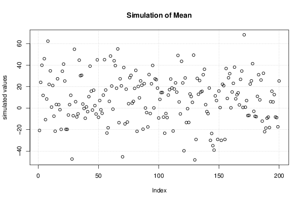
bitmap(file='plot1.png')
plot(r$t[,1],type='p',ylab='simulated values',main='Simulation of Mean')
grid()
dev.off()
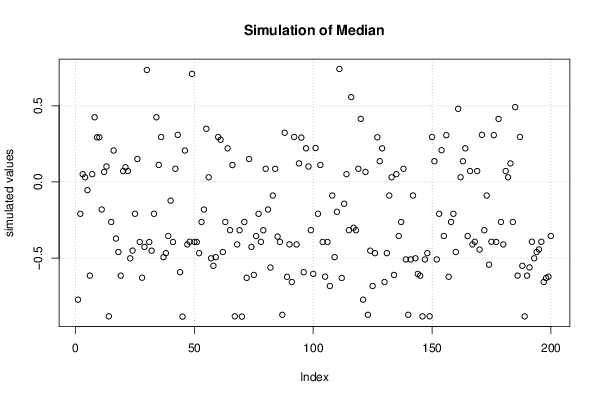
bitmap(file='plot2.png')
plot(r$t[,2],type='p',ylab='simulated values',main='Simulation of Median')
grid()
dev.off()
bitmap(file='plot3.png')
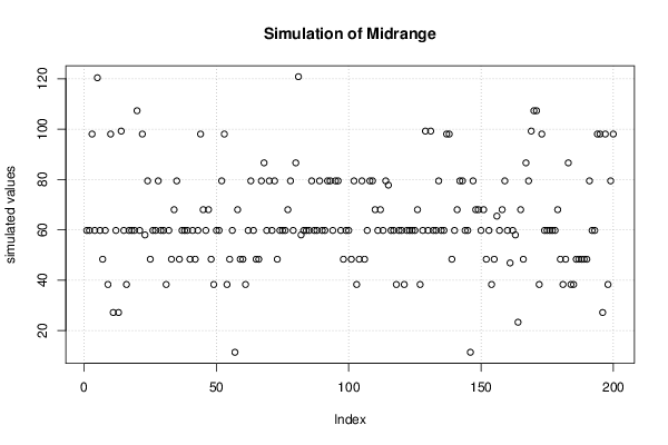
plot(r$t[,3],type='p',ylab='simulated values',main='Simulation of Midrange')
grid()
dev.off()
bitmap(file='plot7.png')
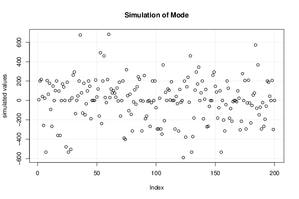
plot(r$t[,4],type='p',ylab='simulated values',main='Simulation of Mode')
grid()
dev.off()
bitmap(file='plot8.png')
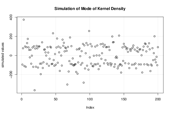
plot(r$t[,5],type='p',ylab='simulated values',main='Simulation of Mode of Kernel Density')
grid()
dev.off()
bitmap(file='plot4.png')
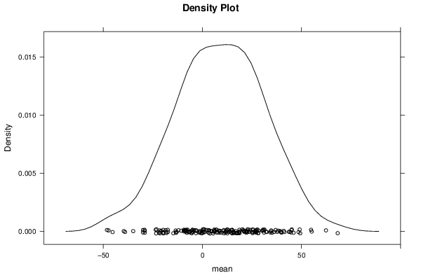
densityplot(~r$t[,1],col='black',main='Density Plot',xlab='mean')
dev.off()
bitmap(file='plot5.png')
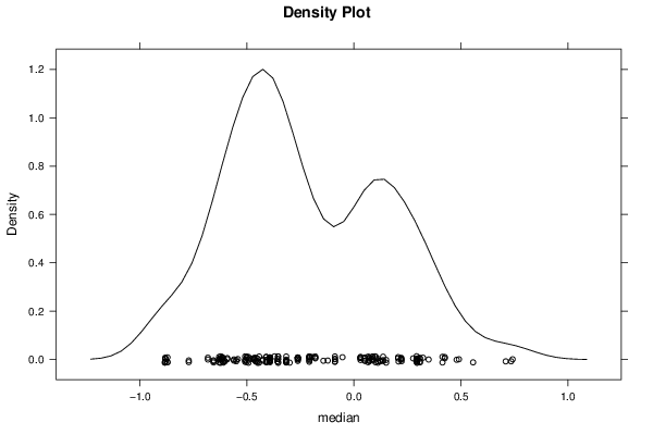
densityplot(~r$t[,2],col='black',main='Density Plot',xlab='median')
dev.off()
bitmap(file='plot6.png')
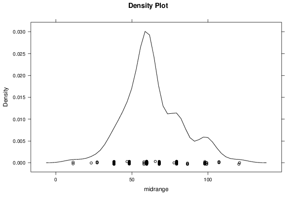
densityplot(~r$t[,3],col='black',main='Density Plot',xlab='midrange')
dev.off()
bitmap(file='plot9.png')
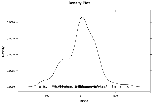
densityplot(~r$t[,4],col='black',main='Density Plot',xlab='mode')
dev.off()
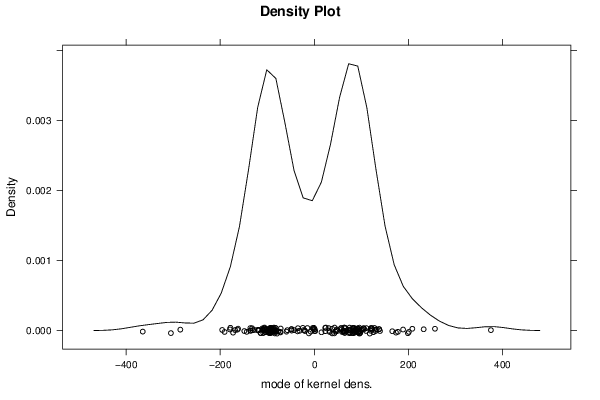
bitmap(file='plot10.png')
densityplot(~r$t[,5],col='black',main='Density Plot',xlab='mode of kernel dens.')
dev.off()
z <- data.frame(cbind(r$t[,1],r$t[,2],r$t[,3],r$t[,4],r$t[,5]))
colnames(z) <- list('mean','median','midrange','mode','mode k.dens')
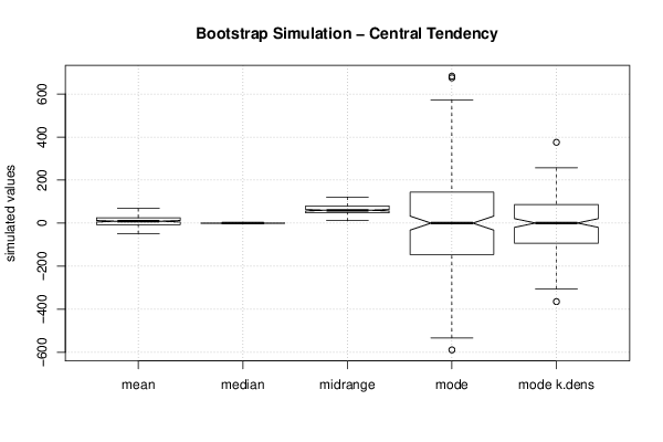
bitmap(file='plot11.png')
boxplot(z,notch=TRUE,ylab='simulated values',main='Bootstrap Simulation - Central Tendency')
grid()
dev.off()
load(file='createtable')
a<-table.start()
a<-table.row.start(a)
a<-table.element(a,'Estimation Results of Bootstrap',10,TRUE)
a<-table.row.end(a)
if (par4 == 'P1 P5 Q1 Q3 P95 P99') {
myq.1 <- 0.01
myq.2 <- 0.05
myq.3 <- 0.95
myq.4 <- 0.99
myl.1 <- 'P1'
myl.2 <- 'P5'
myl.3 <- 'P95'
myl.4 <- 'P99'
}
if (par4 == 'P0.5 P2.5 Q1 Q3 P97.5 P99.5') {
myq.1 <- 0.005
myq.2 <- 0.025
myq.3 <- 0.975
myq.4 <- 0.995
myl.1 <- 'P0.5'
myl.2 <- 'P2.5'
myl.3 <- 'P97.5'
myl.4 <- 'P99.5'
}
if (par4 == 'P10 P20 Q1 Q3 P80 P90') {
myq.1 <- 0.10
myq.2 <- 0.20
myq.3 <- 0.80
myq.4 <- 0.90
myl.1 <- 'P10'
myl.2 <- 'P20'
myl.3 <- 'P80'
myl.4 <- 'P90'
}
a<-table.row.start(a)
a<-table.element(a,'statistic',header=TRUE)
a<-table.element(a,myl.1,header=TRUE)
a<-table.element(a,myl.2,header=TRUE)
a<-table.element(a,'Q1',header=TRUE)
a<-table.element(a,'Estimate',header=TRUE)
a<-table.element(a,'Q3',header=TRUE)
a<-table.element(a,myl.3,header=TRUE)
a<-table.element(a,myl.4,header=TRUE)
a<-table.element(a,'S.D.',header=TRUE)
a<-table.element(a,'IQR',header=TRUE)
a<-table.row.end(a)
a<-table.row.start(a)
a<-table.element(a,'mean',header=TRUE)
q1 <- quantile(r$t[,1],0.25)[[1]]
q3 <- quantile(r$t[,1],0.75)[[1]]
p01 <- quantile(r$t[,1],myq.1)[[1]]
p05 <- quantile(r$t[,1],myq.2)[[1]]
p95 <- quantile(r$t[,1],myq.3)[[1]]
p99 <- quantile(r$t[,1],myq.4)[[1]]
a<-table.element(a,signif(p01,par2))
a<-table.element(a,signif(p05,par2))
a<-table.element(a,signif(q1,par2))
a<-table.element(a,signif(r$t0[1],par2))
a<-table.element(a,signif(q3,par2))
a<-table.element(a,signif(p95,par2))
a<-table.element(a,signif(p99,par2))
a<-table.element( a,signif( sqrt(var(r$t[,1])),par2 ) )
a<-table.element(a,signif(q3-q1,par2))
a<-table.row.end(a)
a<-table.row.start(a)
a<-table.element(a,'median',header=TRUE)
q1 <- quantile(r$t[,2],0.25)[[1]]
q3 <- quantile(r$t[,2],0.75)[[1]]
p01 <- quantile(r$t[,2],myq.1)[[1]]
p05 <- quantile(r$t[,2],myq.2)[[1]]
p95 <- quantile(r$t[,2],myq.3)[[1]]
p99 <- quantile(r$t[,2],myq.4)[[1]]
a<-table.element(a,signif(p01,par2))
a<-table.element(a,signif(p05,par2))
a<-table.element(a,signif(q1,par2))
a<-table.element(a,signif(r$t0[2],par2))
a<-table.element(a,signif(q3,par2))
a<-table.element(a,signif(p95,par2))
a<-table.element(a,signif(p99,par2))
a<-table.element(a,signif(sqrt(var(r$t[,2])),par2))
a<-table.element(a,signif(q3-q1,par2))
a<-table.row.end(a)
a<-table.row.start(a)
a<-table.element(a,'midrange',header=TRUE)
q1 <- quantile(r$t[,3],0.25)[[1]]
q3 <- quantile(r$t[,3],0.75)[[1]]
p01 <- quantile(r$t[,3],myq.1)[[1]]
p05 <- quantile(r$t[,3],myq.2)[[1]]
p95 <- quantile(r$t[,3],myq.3)[[1]]
p99 <- quantile(r$t[,3],myq.4)[[1]]
a<-table.element(a,signif(p01,par2))
a<-table.element(a,signif(p05,par2))
a<-table.element(a,signif(q1,par2))
a<-table.element(a,signif(r$t0[3],par2))
a<-table.element(a,signif(q3,par2))
a<-table.element(a,signif(p95,par2))
a<-table.element(a,signif(p99,par2))
a<-table.element(a,signif(sqrt(var(r$t[,3])),par2))
a<-table.element(a,signif(q3-q1,par2))
a<-table.row.end(a)
a<-table.row.start(a)
a<-table.element(a,'mode',header=TRUE)
q1 <- quantile(r$t[,4],0.25)[[1]]
q3 <- quantile(r$t[,4],0.75)[[1]]
p01 <- quantile(r$t[,4],myq.1)[[1]]
p05 <- quantile(r$t[,4],myq.2)[[1]]
p95 <- quantile(r$t[,4],myq.3)[[1]]
p99 <- quantile(r$t[,4],myq.4)[[1]]
a<-table.element(a,signif(p01,par2))
a<-table.element(a,signif(p05,par2))
a<-table.element(a,signif(q1,par2))
a<-table.element(a,signif(r$t0[4],par2))
a<-table.element(a,signif(q3,par2))
a<-table.element(a,signif(p95,par2))
a<-table.element(a,signif(p99,par2))
a<-table.element(a,signif(sqrt(var(r$t[,4])),par2))
a<-table.element(a,signif(q3-q1,par2))
a<-table.row.end(a)
a<-table.row.start(a)
a<-table.element(a,'mode k.dens',header=TRUE)
q1 <- quantile(r$t[,5],0.25)[[1]]
q3 <- quantile(r$t[,5],0.75)[[1]]
p01 <- quantile(r$t[,5],myq.1)[[1]]
p05 <- quantile(r$t[,5],myq.2)[[1]]
p95 <- quantile(r$t[,5],myq.3)[[1]]
p99 <- quantile(r$t[,5],myq.4)[[1]]
a<-table.element(a,signif(p01,par2))
a<-table.element(a,signif(p05,par2))
a<-table.element(a,signif(q1,par2))
a<-table.element(a,signif(r$t0[5],par2))
a<-table.element(a,signif(q3,par2))
a<-table.element(a,signif(p95,par2))
a<-table.element(a,signif(p99,par2))
a<-table.element(a,signif(sqrt(var(r$t[,5])),par2))
a<-table.element(a,signif(q3-q1,par2))
a<-table.row.end(a)
a<-table.end(a)
table.save(a,file='mytable.tab')