Repository of Reproducible Computations

Free Statistics

of Irreproducible Research!

Author's title

Author

*Unverified author*

R Software Module

rwasp_autocorrelation.wasp

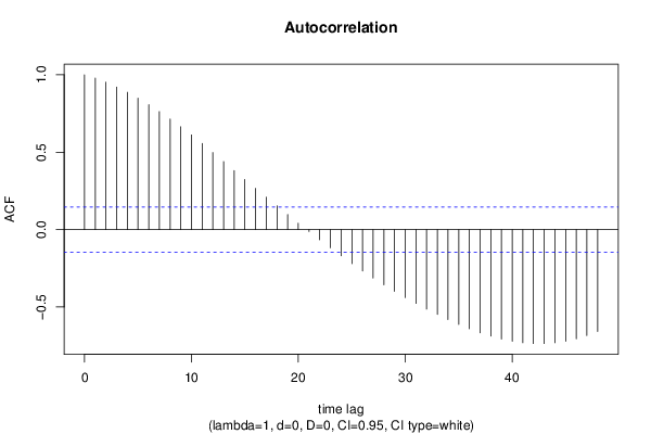
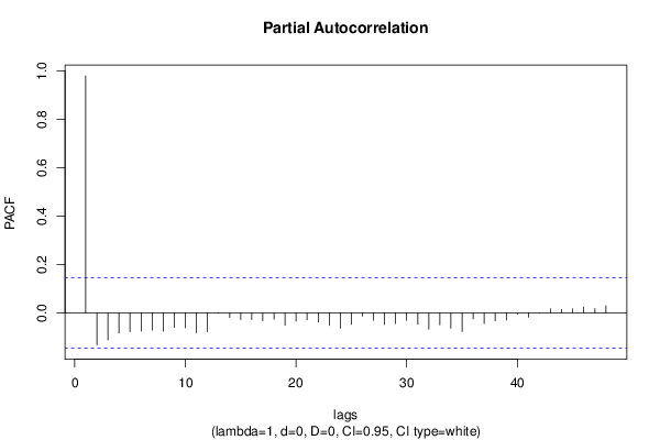
Title produced by software

(Partial) Autocorrelation Function

Date of computation

Thu, 13 Mar 2014 09:17:36 -0400

Cite this page as follows

Statistical Computations at FreeStatistics.org, Office for Research Development and Education, URL https://freestatistics.org/blog/index.php?v=date/2014/Mar/13/t1394716665ecooxvjzgwr5xwp.htm/, Retrieved Tue, 14 May 2024 23:49:37 +0000

Statistical Computations at FreeStatistics.org, Office for Research Development and Education, URL https://freestatistics.org/blog/index.php?pk=234223, Retrieved Tue, 14 May 2024 23:49:37 +0000

QR Codes:

Paste this QR Code to cite your computation.

Original text written by user:

IsPrivate?

No (this computation is public)

User-defined keywords

Estimated Impact

148

Family? (F = Feedback message, R = changed R code, M = changed R Module, P = changed Parameters, D = changed Data)

-       [(Partial) Autocorrelation Function] [] [2014-03-13 13:17:36] [a17c9baa293c9bc97942594e3a0541eb] [Current]

Feedback Forum

Post a new message

Dataseries X:

Download CSV

Histogram

Boxplots

Summary of computational transaction
Raw Input	view raw input (R code)
Raw Output	view raw output of R engine
Computing time	3 seconds
R Server	'Gwilym Jenkins' @ jenkins.wessa.net

\begin{tabular}{lllllllll}
\hline
Summary of computational transaction \tabularnewline
Raw Input & view raw input (R code)  \tabularnewline
Raw Output & view raw output of R engine  \tabularnewline
Computing time & 3 seconds \tabularnewline
R Server & 'Gwilym Jenkins' @ jenkins.wessa.net \tabularnewline
\hline
\end{tabular}
%Source: https://freestatistics.org/blog/index.php?pk=234223&T=0

[TABLE]
[ROW][C]Summary of computational transaction[/C][/ROW]
[ROW][C]Raw Input[/C][C]view raw input (R code) [/C][/ROW]
[ROW][C]Raw Output[/C][C]view raw output of R engine [/C][/ROW]
[ROW][C]Computing time[/C][C]3 seconds[/C][/ROW]
[ROW][C]R Server[/C][C]'Gwilym Jenkins' @ jenkins.wessa.net[/C][/ROW]
[/TABLE]
Source: https://freestatistics.org/blog/index.php?pk=234223&T=0

Globally Unique Identifier (entire table): ba.freestatistics.org/blog/index.php?pk=234223&T=0

As an alternative you can also use a QR Code:

The GUIDs for individual cells are displayed in the table below:

Summary of computational transaction
Raw Input	view raw input (R code)
Raw Output	view raw output of R engine
Computing time	3 seconds
R Server	'Gwilym Jenkins' @ jenkins.wessa.net

Autocorrelation Function
Time lag k	ACF(k)	T-STAT	P-value
1	0.978739	13.1312	0
2	0.952368	12.7774	0
3	0.921341	12.3611	0
4	0.886631	11.8954	0
5	0.848464	11.3833	0
6	0.806983	10.8268	0
7	0.762419	10.2289	0
8	0.714653	9.5881	0
9	0.664372	8.9135	0
10	0.611707	8.2069	0
11	0.556009	7.4596	0
12	0.497579	6.6757	0
13	0.439552	5.8972	0
14	0.381645	5.1203	0
15	0.323886	4.3454	1.2e-05
16	0.266463	3.575	0.000225
17	0.209413	2.8096	0.002755
18	0.153158	2.0548	0.02067
19	0.096956	1.3008	0.097495
20	0.041646	0.5587	0.288516
21	-0.01242	-0.1666	0.433925
22	-0.0654	-0.8774	0.190709
23	-0.117543	-1.577	0.058275
24	-0.169129	-2.2691	0.012224
25	-0.219541	-2.9455	0.001826
26	-0.267368	-3.5871	0.000215
27	-0.313037	-4.1998	2.1e-05
28	-0.357078	-4.7907	2e-06
29	-0.399309	-5.3573	0
30	-0.439189	-5.8923	0
31	-0.477075	-6.4006	0
32	-0.513633	-6.8911	0
33	-0.548168	-7.3545	0
34	-0.581153	-7.797	0
35	-0.612912	-8.2231	0
36	-0.641178	-8.6023	0
37	-0.666485	-8.9418	0
38	-0.688459	-9.2366	0
39	-0.706968	-9.485	0
40	-0.72095	-9.6726	0
41	-0.730855	-9.8055	0
42	-0.736196	-9.8771	0
43	-0.736293	-9.8784	0
44	-0.731177	-9.8098	0
45	-0.720912	-9.6721	0
46	-0.705322	-9.4629	0
47	-0.68464	-9.1854	0
48	-0.658755	-8.8381	0

\begin{tabular}{lllllllll}
\hline
Autocorrelation Function \tabularnewline
Time lag k & ACF(k) & T-STAT & P-value \tabularnewline
1 & 0.978739 & 13.1312 & 0 \tabularnewline
2 & 0.952368 & 12.7774 & 0 \tabularnewline
3 & 0.921341 & 12.3611 & 0 \tabularnewline
4 & 0.886631 & 11.8954 & 0 \tabularnewline
5 & 0.848464 & 11.3833 & 0 \tabularnewline
6 & 0.806983 & 10.8268 & 0 \tabularnewline
7 & 0.762419 & 10.2289 & 0 \tabularnewline
8 & 0.714653 & 9.5881 & 0 \tabularnewline
9 & 0.664372 & 8.9135 & 0 \tabularnewline
10 & 0.611707 & 8.2069 & 0 \tabularnewline
11 & 0.556009 & 7.4596 & 0 \tabularnewline
12 & 0.497579 & 6.6757 & 0 \tabularnewline
13 & 0.439552 & 5.8972 & 0 \tabularnewline
14 & 0.381645 & 5.1203 & 0 \tabularnewline
15 & 0.323886 & 4.3454 & 1.2e-05 \tabularnewline
16 & 0.266463 & 3.575 & 0.000225 \tabularnewline
17 & 0.209413 & 2.8096 & 0.002755 \tabularnewline
18 & 0.153158 & 2.0548 & 0.02067 \tabularnewline
19 & 0.096956 & 1.3008 & 0.097495 \tabularnewline
20 & 0.041646 & 0.5587 & 0.288516 \tabularnewline
21 & -0.01242 & -0.1666 & 0.433925 \tabularnewline
22 & -0.0654 & -0.8774 & 0.190709 \tabularnewline
23 & -0.117543 & -1.577 & 0.058275 \tabularnewline
24 & -0.169129 & -2.2691 & 0.012224 \tabularnewline
25 & -0.219541 & -2.9455 & 0.001826 \tabularnewline
26 & -0.267368 & -3.5871 & 0.000215 \tabularnewline
27 & -0.313037 & -4.1998 & 2.1e-05 \tabularnewline
28 & -0.357078 & -4.7907 & 2e-06 \tabularnewline
29 & -0.399309 & -5.3573 & 0 \tabularnewline
30 & -0.439189 & -5.8923 & 0 \tabularnewline
31 & -0.477075 & -6.4006 & 0 \tabularnewline
32 & -0.513633 & -6.8911 & 0 \tabularnewline
33 & -0.548168 & -7.3545 & 0 \tabularnewline
34 & -0.581153 & -7.797 & 0 \tabularnewline
35 & -0.612912 & -8.2231 & 0 \tabularnewline
36 & -0.641178 & -8.6023 & 0 \tabularnewline
37 & -0.666485 & -8.9418 & 0 \tabularnewline
38 & -0.688459 & -9.2366 & 0 \tabularnewline
39 & -0.706968 & -9.485 & 0 \tabularnewline
40 & -0.72095 & -9.6726 & 0 \tabularnewline
41 & -0.730855 & -9.8055 & 0 \tabularnewline
42 & -0.736196 & -9.8771 & 0 \tabularnewline
43 & -0.736293 & -9.8784 & 0 \tabularnewline
44 & -0.731177 & -9.8098 & 0 \tabularnewline
45 & -0.720912 & -9.6721 & 0 \tabularnewline
46 & -0.705322 & -9.4629 & 0 \tabularnewline
47 & -0.68464 & -9.1854 & 0 \tabularnewline
48 & -0.658755 & -8.8381 & 0 \tabularnewline
\hline
\end{tabular}
%Source: https://freestatistics.org/blog/index.php?pk=234223&T=1

[TABLE]
[ROW][C]Autocorrelation Function[/C][/ROW]
[ROW][C]Time lag k[/C][C]ACF(k)[/C][C]T-STAT[/C][C]P-value[/C][/ROW]
[ROW][C]1[/C][C]0.978739[/C][C]13.1312[/C][C]0[/C][/ROW]
[ROW][C]2[/C][C]0.952368[/C][C]12.7774[/C][C]0[/C][/ROW]
[ROW][C]3[/C][C]0.921341[/C][C]12.3611[/C][C]0[/C][/ROW]
[ROW][C]4[/C][C]0.886631[/C][C]11.8954[/C][C]0[/C][/ROW]
[ROW][C]5[/C][C]0.848464[/C][C]11.3833[/C][C]0[/C][/ROW]
[ROW][C]6[/C][C]0.806983[/C][C]10.8268[/C][C]0[/C][/ROW]
[ROW][C]7[/C][C]0.762419[/C][C]10.2289[/C][C]0[/C][/ROW]
[ROW][C]8[/C][C]0.714653[/C][C]9.5881[/C][C]0[/C][/ROW]
[ROW][C]9[/C][C]0.664372[/C][C]8.9135[/C][C]0[/C][/ROW]
[ROW][C]10[/C][C]0.611707[/C][C]8.2069[/C][C]0[/C][/ROW]
[ROW][C]11[/C][C]0.556009[/C][C]7.4596[/C][C]0[/C][/ROW]
[ROW][C]12[/C][C]0.497579[/C][C]6.6757[/C][C]0[/C][/ROW]
[ROW][C]13[/C][C]0.439552[/C][C]5.8972[/C][C]0[/C][/ROW]
[ROW][C]14[/C][C]0.381645[/C][C]5.1203[/C][C]0[/C][/ROW]
[ROW][C]15[/C][C]0.323886[/C][C]4.3454[/C][C]1.2e-05[/C][/ROW]
[ROW][C]16[/C][C]0.266463[/C][C]3.575[/C][C]0.000225[/C][/ROW]
[ROW][C]17[/C][C]0.209413[/C][C]2.8096[/C][C]0.002755[/C][/ROW]
[ROW][C]18[/C][C]0.153158[/C][C]2.0548[/C][C]0.02067[/C][/ROW]
[ROW][C]19[/C][C]0.096956[/C][C]1.3008[/C][C]0.097495[/C][/ROW]
[ROW][C]20[/C][C]0.041646[/C][C]0.5587[/C][C]0.288516[/C][/ROW]
[ROW][C]21[/C][C]-0.01242[/C][C]-0.1666[/C][C]0.433925[/C][/ROW]
[ROW][C]22[/C][C]-0.0654[/C][C]-0.8774[/C][C]0.190709[/C][/ROW]
[ROW][C]23[/C][C]-0.117543[/C][C]-1.577[/C][C]0.058275[/C][/ROW]
[ROW][C]24[/C][C]-0.169129[/C][C]-2.2691[/C][C]0.012224[/C][/ROW]
[ROW][C]25[/C][C]-0.219541[/C][C]-2.9455[/C][C]0.001826[/C][/ROW]
[ROW][C]26[/C][C]-0.267368[/C][C]-3.5871[/C][C]0.000215[/C][/ROW]
[ROW][C]27[/C][C]-0.313037[/C][C]-4.1998[/C][C]2.1e-05[/C][/ROW]
[ROW][C]28[/C][C]-0.357078[/C][C]-4.7907[/C][C]2e-06[/C][/ROW]
[ROW][C]29[/C][C]-0.399309[/C][C]-5.3573[/C][C]0[/C][/ROW]
[ROW][C]30[/C][C]-0.439189[/C][C]-5.8923[/C][C]0[/C][/ROW]
[ROW][C]31[/C][C]-0.477075[/C][C]-6.4006[/C][C]0[/C][/ROW]
[ROW][C]32[/C][C]-0.513633[/C][C]-6.8911[/C][C]0[/C][/ROW]
[ROW][C]33[/C][C]-0.548168[/C][C]-7.3545[/C][C]0[/C][/ROW]
[ROW][C]34[/C][C]-0.581153[/C][C]-7.797[/C][C]0[/C][/ROW]
[ROW][C]35[/C][C]-0.612912[/C][C]-8.2231[/C][C]0[/C][/ROW]
[ROW][C]36[/C][C]-0.641178[/C][C]-8.6023[/C][C]0[/C][/ROW]
[ROW][C]37[/C][C]-0.666485[/C][C]-8.9418[/C][C]0[/C][/ROW]
[ROW][C]38[/C][C]-0.688459[/C][C]-9.2366[/C][C]0[/C][/ROW]
[ROW][C]39[/C][C]-0.706968[/C][C]-9.485[/C][C]0[/C][/ROW]
[ROW][C]40[/C][C]-0.72095[/C][C]-9.6726[/C][C]0[/C][/ROW]
[ROW][C]41[/C][C]-0.730855[/C][C]-9.8055[/C][C]0[/C][/ROW]
[ROW][C]42[/C][C]-0.736196[/C][C]-9.8771[/C][C]0[/C][/ROW]
[ROW][C]43[/C][C]-0.736293[/C][C]-9.8784[/C][C]0[/C][/ROW]
[ROW][C]44[/C][C]-0.731177[/C][C]-9.8098[/C][C]0[/C][/ROW]
[ROW][C]45[/C][C]-0.720912[/C][C]-9.6721[/C][C]0[/C][/ROW]
[ROW][C]46[/C][C]-0.705322[/C][C]-9.4629[/C][C]0[/C][/ROW]
[ROW][C]47[/C][C]-0.68464[/C][C]-9.1854[/C][C]0[/C][/ROW]
[ROW][C]48[/C][C]-0.658755[/C][C]-8.8381[/C][C]0[/C][/ROW]
[/TABLE]
Source: https://freestatistics.org/blog/index.php?pk=234223&T=1

Globally Unique Identifier (entire table): ba.freestatistics.org/blog/index.php?pk=234223&T=1

As an alternative you can also use a QR Code:

The GUIDs for individual cells are displayed in the table below:

Autocorrelation Function
Time lag k	ACF(k)	T-STAT	P-value
1	0.978739	13.1312	0
2	0.952368	12.7774	0
3	0.921341	12.3611	0
4	0.886631	11.8954	0
5	0.848464	11.3833	0
6	0.806983	10.8268	0
7	0.762419	10.2289	0
8	0.714653	9.5881	0
9	0.664372	8.9135	0
10	0.611707	8.2069	0
11	0.556009	7.4596	0
12	0.497579	6.6757	0
13	0.439552	5.8972	0
14	0.381645	5.1203	0
15	0.323886	4.3454	1.2e-05
16	0.266463	3.575	0.000225
17	0.209413	2.8096	0.002755
18	0.153158	2.0548	0.02067
19	0.096956	1.3008	0.097495
20	0.041646	0.5587	0.288516
21	-0.01242	-0.1666	0.433925
22	-0.0654	-0.8774	0.190709
23	-0.117543	-1.577	0.058275
24	-0.169129	-2.2691	0.012224
25	-0.219541	-2.9455	0.001826
26	-0.267368	-3.5871	0.000215
27	-0.313037	-4.1998	2.1e-05
28	-0.357078	-4.7907	2e-06
29	-0.399309	-5.3573	0
30	-0.439189	-5.8923	0
31	-0.477075	-6.4006	0
32	-0.513633	-6.8911	0
33	-0.548168	-7.3545	0
34	-0.581153	-7.797	0
35	-0.612912	-8.2231	0
36	-0.641178	-8.6023	0
37	-0.666485	-8.9418	0
38	-0.688459	-9.2366	0
39	-0.706968	-9.485	0
40	-0.72095	-9.6726	0
41	-0.730855	-9.8055	0
42	-0.736196	-9.8771	0
43	-0.736293	-9.8784	0
44	-0.731177	-9.8098	0
45	-0.720912	-9.6721	0
46	-0.705322	-9.4629	0
47	-0.68464	-9.1854	0
48	-0.658755	-8.8381	0

Partial Autocorrelation Function
Time lag k	PACF(k)	T-STAT	P-value
1	0.978739	13.1312	0
2	-0.132202	-1.7737	0.038903
3	-0.111654	-1.498	0.067943
4	-0.082916	-1.1124	0.133718
5	-0.077399	-1.0384	0.150235
6	-0.074869	-1.0045	0.158251
7	-0.070353	-0.9439	0.173246
8	-0.075534	-1.0134	0.156114
9	-0.060252	-0.8084	0.209975
10	-0.061126	-0.8201	0.206626
11	-0.08217	-1.1024	0.135875
12	-0.077157	-1.0352	0.150988
13	-0.000713	-0.0096	0.496188
14	-0.019334	-0.2594	0.397812
15	-0.027236	-0.3654	0.357616
16	-0.027347	-0.3669	0.357065
17	-0.031603	-0.424	0.336037
18	-0.025683	-0.3446	0.365407
19	-0.05054	-0.6781	0.249301
20	-0.033922	-0.4551	0.324788
21	-0.028297	-0.3796	0.352326
22	-0.037634	-0.5049	0.307119
23	-0.051471	-0.6906	0.245366
24	-0.064088	-0.8598	0.195513
25	-0.04737	-0.6355	0.262945
26	-0.01317	-0.1767	0.429976
27	-0.030484	-0.409	0.34152
28	-0.048025	-0.6443	0.260095
29	-0.043736	-0.5868	0.279045
30	-0.03067	-0.4115	0.340603
31	-0.046789	-0.6277	0.265483
32	-0.06693	-0.898	0.185203
33	-0.048914	-0.6563	0.256249
34	-0.063132	-0.847	0.199059
35	-0.076847	-1.031	0.151958
36	-0.024646	-0.3307	0.370645
37	-0.043909	-0.5891	0.278266
38	-0.032885	-0.4412	0.329798
39	-0.029605	-0.3972	0.34585
40	-0.004957	-0.0665	0.473526
41	-0.017653	-0.2368	0.406527
42	-0.001112	-0.0149	0.494054
43	0.016846	0.226	0.410726
44	0.014155	0.1899	0.424796
45	0.017247	0.2314	0.408638
46	0.024196	0.3246	0.372921
47	0.018001	0.2415	0.404718
48	0.029531	0.3962	0.346211

\begin{tabular}{lllllllll}
\hline
Partial Autocorrelation Function \tabularnewline
Time lag k & PACF(k) & T-STAT & P-value \tabularnewline
1 & 0.978739 & 13.1312 & 0 \tabularnewline
2 & -0.132202 & -1.7737 & 0.038903 \tabularnewline
3 & -0.111654 & -1.498 & 0.067943 \tabularnewline
4 & -0.082916 & -1.1124 & 0.133718 \tabularnewline
5 & -0.077399 & -1.0384 & 0.150235 \tabularnewline
6 & -0.074869 & -1.0045 & 0.158251 \tabularnewline
7 & -0.070353 & -0.9439 & 0.173246 \tabularnewline
8 & -0.075534 & -1.0134 & 0.156114 \tabularnewline
9 & -0.060252 & -0.8084 & 0.209975 \tabularnewline
10 & -0.061126 & -0.8201 & 0.206626 \tabularnewline
11 & -0.08217 & -1.1024 & 0.135875 \tabularnewline
12 & -0.077157 & -1.0352 & 0.150988 \tabularnewline
13 & -0.000713 & -0.0096 & 0.496188 \tabularnewline
14 & -0.019334 & -0.2594 & 0.397812 \tabularnewline
15 & -0.027236 & -0.3654 & 0.357616 \tabularnewline
16 & -0.027347 & -0.3669 & 0.357065 \tabularnewline
17 & -0.031603 & -0.424 & 0.336037 \tabularnewline
18 & -0.025683 & -0.3446 & 0.365407 \tabularnewline
19 & -0.05054 & -0.6781 & 0.249301 \tabularnewline
20 & -0.033922 & -0.4551 & 0.324788 \tabularnewline
21 & -0.028297 & -0.3796 & 0.352326 \tabularnewline
22 & -0.037634 & -0.5049 & 0.307119 \tabularnewline
23 & -0.051471 & -0.6906 & 0.245366 \tabularnewline
24 & -0.064088 & -0.8598 & 0.195513 \tabularnewline
25 & -0.04737 & -0.6355 & 0.262945 \tabularnewline
26 & -0.01317 & -0.1767 & 0.429976 \tabularnewline
27 & -0.030484 & -0.409 & 0.34152 \tabularnewline
28 & -0.048025 & -0.6443 & 0.260095 \tabularnewline
29 & -0.043736 & -0.5868 & 0.279045 \tabularnewline
30 & -0.03067 & -0.4115 & 0.340603 \tabularnewline
31 & -0.046789 & -0.6277 & 0.265483 \tabularnewline
32 & -0.06693 & -0.898 & 0.185203 \tabularnewline
33 & -0.048914 & -0.6563 & 0.256249 \tabularnewline
34 & -0.063132 & -0.847 & 0.199059 \tabularnewline
35 & -0.076847 & -1.031 & 0.151958 \tabularnewline
36 & -0.024646 & -0.3307 & 0.370645 \tabularnewline
37 & -0.043909 & -0.5891 & 0.278266 \tabularnewline
38 & -0.032885 & -0.4412 & 0.329798 \tabularnewline
39 & -0.029605 & -0.3972 & 0.34585 \tabularnewline
40 & -0.004957 & -0.0665 & 0.473526 \tabularnewline
41 & -0.017653 & -0.2368 & 0.406527 \tabularnewline
42 & -0.001112 & -0.0149 & 0.494054 \tabularnewline
43 & 0.016846 & 0.226 & 0.410726 \tabularnewline
44 & 0.014155 & 0.1899 & 0.424796 \tabularnewline
45 & 0.017247 & 0.2314 & 0.408638 \tabularnewline
46 & 0.024196 & 0.3246 & 0.372921 \tabularnewline
47 & 0.018001 & 0.2415 & 0.404718 \tabularnewline
48 & 0.029531 & 0.3962 & 0.346211 \tabularnewline
\hline
\end{tabular}
%Source: https://freestatistics.org/blog/index.php?pk=234223&T=2

[TABLE]
[ROW][C]Partial Autocorrelation Function[/C][/ROW]
[ROW][C]Time lag k[/C][C]PACF(k)[/C][C]T-STAT[/C][C]P-value[/C][/ROW]
[ROW][C]1[/C][C]0.978739[/C][C]13.1312[/C][C]0[/C][/ROW]
[ROW][C]2[/C][C]-0.132202[/C][C]-1.7737[/C][C]0.038903[/C][/ROW]
[ROW][C]3[/C][C]-0.111654[/C][C]-1.498[/C][C]0.067943[/C][/ROW]
[ROW][C]4[/C][C]-0.082916[/C][C]-1.1124[/C][C]0.133718[/C][/ROW]
[ROW][C]5[/C][C]-0.077399[/C][C]-1.0384[/C][C]0.150235[/C][/ROW]
[ROW][C]6[/C][C]-0.074869[/C][C]-1.0045[/C][C]0.158251[/C][/ROW]
[ROW][C]7[/C][C]-0.070353[/C][C]-0.9439[/C][C]0.173246[/C][/ROW]
[ROW][C]8[/C][C]-0.075534[/C][C]-1.0134[/C][C]0.156114[/C][/ROW]
[ROW][C]9[/C][C]-0.060252[/C][C]-0.8084[/C][C]0.209975[/C][/ROW]
[ROW][C]10[/C][C]-0.061126[/C][C]-0.8201[/C][C]0.206626[/C][/ROW]
[ROW][C]11[/C][C]-0.08217[/C][C]-1.1024[/C][C]0.135875[/C][/ROW]
[ROW][C]12[/C][C]-0.077157[/C][C]-1.0352[/C][C]0.150988[/C][/ROW]
[ROW][C]13[/C][C]-0.000713[/C][C]-0.0096[/C][C]0.496188[/C][/ROW]
[ROW][C]14[/C][C]-0.019334[/C][C]-0.2594[/C][C]0.397812[/C][/ROW]
[ROW][C]15[/C][C]-0.027236[/C][C]-0.3654[/C][C]0.357616[/C][/ROW]
[ROW][C]16[/C][C]-0.027347[/C][C]-0.3669[/C][C]0.357065[/C][/ROW]
[ROW][C]17[/C][C]-0.031603[/C][C]-0.424[/C][C]0.336037[/C][/ROW]
[ROW][C]18[/C][C]-0.025683[/C][C]-0.3446[/C][C]0.365407[/C][/ROW]
[ROW][C]19[/C][C]-0.05054[/C][C]-0.6781[/C][C]0.249301[/C][/ROW]
[ROW][C]20[/C][C]-0.033922[/C][C]-0.4551[/C][C]0.324788[/C][/ROW]
[ROW][C]21[/C][C]-0.028297[/C][C]-0.3796[/C][C]0.352326[/C][/ROW]
[ROW][C]22[/C][C]-0.037634[/C][C]-0.5049[/C][C]0.307119[/C][/ROW]
[ROW][C]23[/C][C]-0.051471[/C][C]-0.6906[/C][C]0.245366[/C][/ROW]
[ROW][C]24[/C][C]-0.064088[/C][C]-0.8598[/C][C]0.195513[/C][/ROW]
[ROW][C]25[/C][C]-0.04737[/C][C]-0.6355[/C][C]0.262945[/C][/ROW]
[ROW][C]26[/C][C]-0.01317[/C][C]-0.1767[/C][C]0.429976[/C][/ROW]
[ROW][C]27[/C][C]-0.030484[/C][C]-0.409[/C][C]0.34152[/C][/ROW]
[ROW][C]28[/C][C]-0.048025[/C][C]-0.6443[/C][C]0.260095[/C][/ROW]
[ROW][C]29[/C][C]-0.043736[/C][C]-0.5868[/C][C]0.279045[/C][/ROW]
[ROW][C]30[/C][C]-0.03067[/C][C]-0.4115[/C][C]0.340603[/C][/ROW]
[ROW][C]31[/C][C]-0.046789[/C][C]-0.6277[/C][C]0.265483[/C][/ROW]
[ROW][C]32[/C][C]-0.06693[/C][C]-0.898[/C][C]0.185203[/C][/ROW]
[ROW][C]33[/C][C]-0.048914[/C][C]-0.6563[/C][C]0.256249[/C][/ROW]
[ROW][C]34[/C][C]-0.063132[/C][C]-0.847[/C][C]0.199059[/C][/ROW]
[ROW][C]35[/C][C]-0.076847[/C][C]-1.031[/C][C]0.151958[/C][/ROW]
[ROW][C]36[/C][C]-0.024646[/C][C]-0.3307[/C][C]0.370645[/C][/ROW]
[ROW][C]37[/C][C]-0.043909[/C][C]-0.5891[/C][C]0.278266[/C][/ROW]
[ROW][C]38[/C][C]-0.032885[/C][C]-0.4412[/C][C]0.329798[/C][/ROW]
[ROW][C]39[/C][C]-0.029605[/C][C]-0.3972[/C][C]0.34585[/C][/ROW]
[ROW][C]40[/C][C]-0.004957[/C][C]-0.0665[/C][C]0.473526[/C][/ROW]
[ROW][C]41[/C][C]-0.017653[/C][C]-0.2368[/C][C]0.406527[/C][/ROW]
[ROW][C]42[/C][C]-0.001112[/C][C]-0.0149[/C][C]0.494054[/C][/ROW]
[ROW][C]43[/C][C]0.016846[/C][C]0.226[/C][C]0.410726[/C][/ROW]
[ROW][C]44[/C][C]0.014155[/C][C]0.1899[/C][C]0.424796[/C][/ROW]
[ROW][C]45[/C][C]0.017247[/C][C]0.2314[/C][C]0.408638[/C][/ROW]
[ROW][C]46[/C][C]0.024196[/C][C]0.3246[/C][C]0.372921[/C][/ROW]
[ROW][C]47[/C][C]0.018001[/C][C]0.2415[/C][C]0.404718[/C][/ROW]
[ROW][C]48[/C][C]0.029531[/C][C]0.3962[/C][C]0.346211[/C][/ROW]
[/TABLE]
Source: https://freestatistics.org/blog/index.php?pk=234223&T=2

Globally Unique Identifier (entire table): ba.freestatistics.org/blog/index.php?pk=234223&T=2

As an alternative you can also use a QR Code:

The GUIDs for individual cells are displayed in the table below:

Partial Autocorrelation Function
Time lag k	PACF(k)	T-STAT	P-value
1	0.978739	13.1312	0
2	-0.132202	-1.7737	0.038903
3	-0.111654	-1.498	0.067943
4	-0.082916	-1.1124	0.133718
5	-0.077399	-1.0384	0.150235
6	-0.074869	-1.0045	0.158251
7	-0.070353	-0.9439	0.173246
8	-0.075534	-1.0134	0.156114
9	-0.060252	-0.8084	0.209975
10	-0.061126	-0.8201	0.206626
11	-0.08217	-1.1024	0.135875
12	-0.077157	-1.0352	0.150988
13	-0.000713	-0.0096	0.496188
14	-0.019334	-0.2594	0.397812
15	-0.027236	-0.3654	0.357616
16	-0.027347	-0.3669	0.357065
17	-0.031603	-0.424	0.336037
18	-0.025683	-0.3446	0.365407
19	-0.05054	-0.6781	0.249301
20	-0.033922	-0.4551	0.324788
21	-0.028297	-0.3796	0.352326
22	-0.037634	-0.5049	0.307119
23	-0.051471	-0.6906	0.245366
24	-0.064088	-0.8598	0.195513
25	-0.04737	-0.6355	0.262945
26	-0.01317	-0.1767	0.429976
27	-0.030484	-0.409	0.34152
28	-0.048025	-0.6443	0.260095
29	-0.043736	-0.5868	0.279045
30	-0.03067	-0.4115	0.340603
31	-0.046789	-0.6277	0.265483
32	-0.06693	-0.898	0.185203
33	-0.048914	-0.6563	0.256249
34	-0.063132	-0.847	0.199059
35	-0.076847	-1.031	0.151958
36	-0.024646	-0.3307	0.370645
37	-0.043909	-0.5891	0.278266
38	-0.032885	-0.4412	0.329798
39	-0.029605	-0.3972	0.34585
40	-0.004957	-0.0665	0.473526
41	-0.017653	-0.2368	0.406527
42	-0.001112	-0.0149	0.494054
43	0.016846	0.226	0.410726
44	0.014155	0.1899	0.424796
45	0.017247	0.2314	0.408638
46	0.024196	0.3246	0.372921
47	0.018001	0.2415	0.404718
48	0.029531	0.3962	0.346211

Figure 1

PNG link

Postscript link

PDF link

Figure 2

PNG link

Postscript link

PDF link

Figure 3

PNG link

Postscript link

PDF link

Parameters (Session):

par1 = 48 ; par2 = 1 ; par3 = 0 ; par4 = 0 ; par5 = 12 ; par6 = White Noise ; par7 = 0.95 ;

Parameters (R input):

par1 = 48 ; par2 = 1 ; par3 = 0 ; par4 = 0 ; par5 = 12 ; par6 = White Noise ; par7 = 0.95 ; par8 = ;

R code (references can be found in the software module):

if (par1 == 'Default') {
par1 = 10*log10(length(x))
} else {
par1 <- as.numeric(par1)
}
par2 <- as.numeric(par2)
par3 <- as.numeric(par3)
par4 <- as.numeric(par4)
par5 <- as.numeric(par5)
if (par6 == 'White Noise') par6 <- 'white' else par6 <- 'ma'
par7 <- as.numeric(par7)
if (par8 != '') par8 <- as.numeric(par8)
ox <- x
if (par8 == '') {
if (par2 == 0) {
x <- log(x)
} else {
x <- (x ^ par2 - 1) / par2
}
} else {
x <- log(x,base=par8)
}
if (par3 > 0) x <- diff(x,lag=1,difference=par3)
if (par4 > 0) x <- diff(x,lag=par5,difference=par4)
bitmap(file='picts.png')
op <- par(mfrow=c(2,1))
plot(ox,type='l',main='Original Time Series',xlab='time',ylab='value')
if (par8=='') {
mytitle <- paste('Working Time Series (lambda=',par2,', d=',par3,', D=',par4,')',sep='')
mysub <- paste('(lambda=',par2,', d=',par3,', D=',par4,', CI=', par7, ', CI type=',par6,')',sep='')
} else {
mytitle <- paste('Working Time Series (base=',par8,', d=',par3,', D=',par4,')',sep='')
mysub <- paste('(base=',par8,', d=',par3,', D=',par4,', CI=', par7, ', CI type=',par6,')',sep='')
}
plot(x,type='l', main=mytitle,xlab='time',ylab='value')
par(op)
dev.off()
bitmap(file='pic1.png')
racf <- acf(x, par1, main='Autocorrelation', xlab='time lag', ylab='ACF', ci.type=par6, ci=par7, sub=mysub)
dev.off()
bitmap(file='pic2.png')
rpacf <- pacf(x,par1,main='Partial Autocorrelation',xlab='lags',ylab='PACF',sub=mysub)
dev.off()
(myacf <- c(racf$acf))
(mypacf <- c(rpacf$acf))
lengthx <- length(x)
sqrtn <- sqrt(lengthx)
load(file='createtable')
a<-table.start()
a<-table.row.start(a)
a<-table.element(a,'Autocorrelation Function',4,TRUE)
a<-table.row.end(a)
a<-table.row.start(a)
a<-table.element(a,'Time lag k',header=TRUE)
a<-table.element(a,hyperlink('basics.htm','ACF(k)','click here for more information about the Autocorrelation Function'),header=TRUE)
a<-table.element(a,'T-STAT',header=TRUE)
a<-table.element(a,'P-value',header=TRUE)
a<-table.row.end(a)
for (i in 2:(par1+1)) {
a<-table.row.start(a)
a<-table.element(a,i-1,header=TRUE)
a<-table.element(a,round(myacf[i],6))
mytstat <- myacf[i]*sqrtn
a<-table.element(a,round(mytstat,4))
a<-table.element(a,round(1-pt(abs(mytstat),lengthx),6))
a<-table.row.end(a)
}
a<-table.end(a)
table.save(a,file='mytable.tab')
a<-table.start()
a<-table.row.start(a)
a<-table.element(a,'Partial Autocorrelation Function',4,TRUE)
a<-table.row.end(a)
a<-table.row.start(a)
a<-table.element(a,'Time lag k',header=TRUE)
a<-table.element(a,hyperlink('basics.htm','PACF(k)','click here for more information about the Partial Autocorrelation Function'),header=TRUE)
a<-table.element(a,'T-STAT',header=TRUE)
a<-table.element(a,'P-value',header=TRUE)
a<-table.row.end(a)
for (i in 1:par1) {
a<-table.row.start(a)
a<-table.element(a,i,header=TRUE)
a<-table.element(a,round(mypacf[i],6))
mytstat <- mypacf[i]*sqrtn
a<-table.element(a,round(mytstat,4))
a<-table.element(a,round(1-pt(abs(mytstat),lengthx),6))
a<-table.row.end(a)
}
a<-table.end(a)
table.save(a,file='mytable1.tab')

Free Statistics

Description of Statistical Computation

Tree of Dependent Computations

Dataset

Tables (Output of Computation)

Figures (Output of Computation)

Input Parameters & R Code