Free Statistics
of Irreproducible Research!
Description of Statistical Computation | |||||||||||||||||||||
|---|---|---|---|---|---|---|---|---|---|---|---|---|---|---|---|---|---|---|---|---|---|
| Author's title | |||||||||||||||||||||
| Author | *Unverified author* | ||||||||||||||||||||
| R Software Module | rwasp_meanplot.wasp | ||||||||||||||||||||
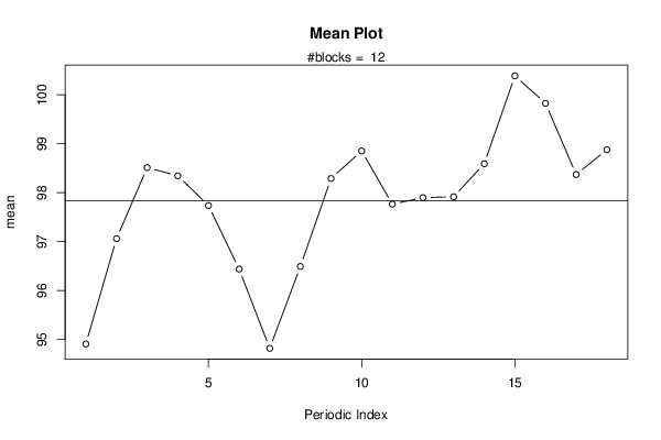
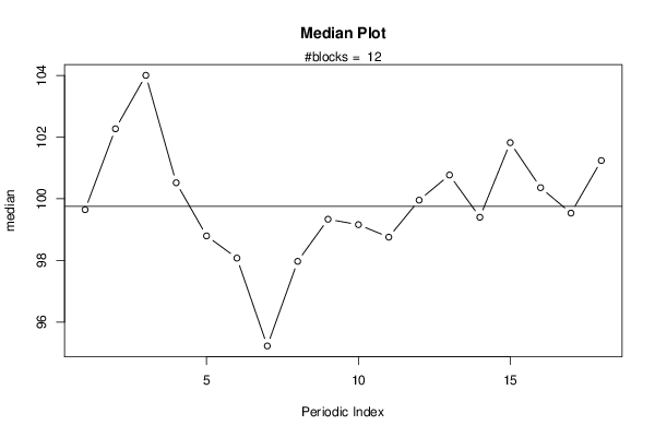
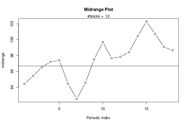
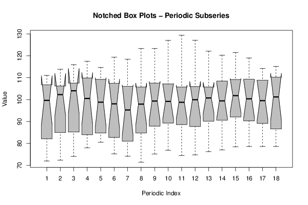
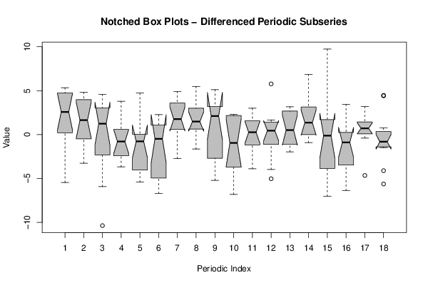
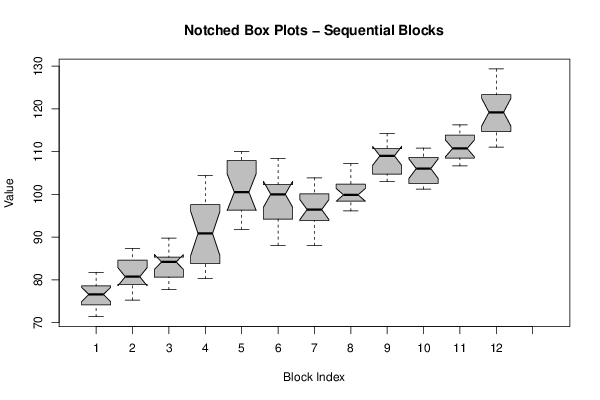
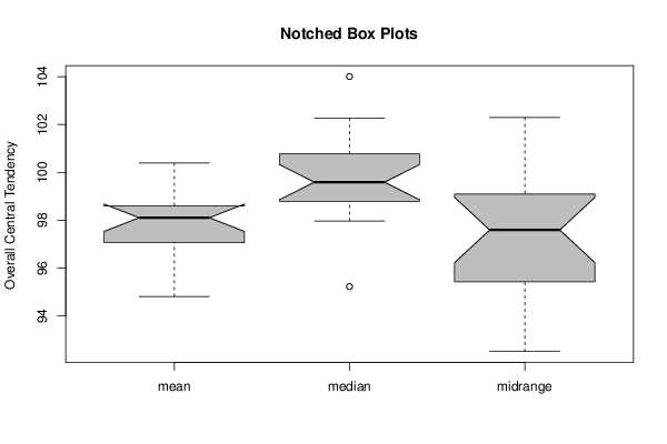
| Title produced by software | Mean Plot | ||||||||||||||||||||
| Date of computation | Mon, 03 Mar 2014 14:53:52 -0500 | ||||||||||||||||||||
| Cite this page as follows | Statistical Computations at FreeStatistics.org, Office for Research Development and Education, URL https://freestatistics.org/blog/index.php?v=date/2014/Mar/03/t1393876459n9ygu7lst5du31a.htm/, Retrieved Tue, 14 May 2024 13:03:26 +0000 | ||||||||||||||||||||
| Statistical Computations at FreeStatistics.org, Office for Research Development and Education, URL https://freestatistics.org/blog/index.php?pk=234154, Retrieved Tue, 14 May 2024 13:03:26 +0000 | |||||||||||||||||||||
| QR Codes: | |||||||||||||||||||||
|
| |||||||||||||||||||||
| Original text written by user: | |||||||||||||||||||||
| IsPrivate? | No (this computation is public) | ||||||||||||||||||||
| User-defined keywords | |||||||||||||||||||||
| Estimated Impact | 120 | ||||||||||||||||||||
Tree of Dependent Computations | |||||||||||||||||||||
| Family? (F = Feedback message, R = changed R code, M = changed R Module, P = changed Parameters, D = changed Data) | |||||||||||||||||||||
| - [Mean Plot] [] [2014-03-03 19:53:52] [7924821bfd3c647737470140bc76edc8] [Current] - R PD [Mean Plot] [] [2014-05-19 18:40:49] [92db97885c79b0659d4d94792fd29e93] | |||||||||||||||||||||
| Feedback Forum | |||||||||||||||||||||
Post a new message | |||||||||||||||||||||
Dataset | |||||||||||||||||||||
| Dataseries X: | |||||||||||||||||||||
71,97 72,32 74,07 77,95 81,75 80,81 74,1 71,37 75,21 76,9 74,44 74,76 76,23 76,97 78,4 78,6 80,08 81,12 80,31 84,59 81,34 80,95 80,48 75,26 76,32 78,92 80,47 83,14 85,42 81,53 87,31 86,01 85,1 79,91 78,6 78,6 79,37 82,89 84,43 85,32 87,71 84,68 80,62 84,79 85,49 81,68 77,69 78,31 79,18 80,91 83,91 86,3 89,76 85,11 83,81 85,36 85,89 82,59 80,87 80,27 81,36 84,81 90,3 95,43 97,59 97,8 99,48 97,52 104,39 97,74 91,37 92,42 96,9 101,58 105,46 110,06 107,9 102,87 96,28 98,59 103,22 98,6 91,79 93,83 95,17 95,19 99,44 109,18 109,15 109,72 108,41 102,96 107,64 97,28 97,25 91,84 94,12 97,86 98,83 102,29 104,49 102,11 102,14 101,28 101,21 94,2 88,47 88,08 88,02 92,95 97,05 101,44 100,34 99,98 94,17 94,54 95,12 98,04 93,72 93,83 93,03 95,81 99,1 100,12 100,67 103,87 102,39 107,21 105,71 99,79 96,12 96,17 97,23 98,08 99,84 99,72 99,92 102,7 102,06 102,36 102,43 100,6 98,4 98,61 103,03 104,7 107,45 109,67 110,54 112,05 113,19 114,2 112,56 107,36 103,93 103,83 104,74 107,5 109,53 109,42 108,6 110,72 105,1 105,19 102,55 101,25 101,56 101,62 101,7 102,94 104,37 106,93 107,82 110,83 106,86 109,46 108,8 108,69 107,77 108,64 108,5 113,84 114,59 116,27 113,63 112,29 110,31 108,47 110,67 109,1 107,02 108,12 106,69 109,87 110,82 114,14 113,31 115,16 111,06 111,13 115,96 117,57 114,69 119,42 118,4 123,32 123,39 127,04 129,35 127,12 122,1 120,22 121,53 119,01 114,27 114,46 | |||||||||||||||||||||
Tables (Output of Computation) | |||||||||||||||||||||
| |||||||||||||||||||||
Figures (Output of Computation) | |||||||||||||||||||||
Input Parameters & R Code | |||||||||||||||||||||
| Parameters (Session): | |||||||||||||||||||||
| par1 = 18 ; | |||||||||||||||||||||
| Parameters (R input): | |||||||||||||||||||||
| par1 = 18 ; | |||||||||||||||||||||
| R code (references can be found in the software module): | |||||||||||||||||||||
par1 <- as.numeric(par1) | |||||||||||||||||||||