Free Statistics
of Irreproducible Research!
Description of Statistical Computation | |||||||||||||||||||||||||||||||||||||||||||||
|---|---|---|---|---|---|---|---|---|---|---|---|---|---|---|---|---|---|---|---|---|---|---|---|---|---|---|---|---|---|---|---|---|---|---|---|---|---|---|---|---|---|---|---|---|---|
| Author's title | |||||||||||||||||||||||||||||||||||||||||||||
| Author | *The author of this computation has been verified* | ||||||||||||||||||||||||||||||||||||||||||||
| R Software Module | rwasp_bidensity.wasp | ||||||||||||||||||||||||||||||||||||||||||||
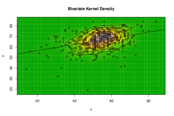
| Title produced by software | Bivariate Kernel Density Estimation | ||||||||||||||||||||||||||||||||||||||||||||
| Date of computation | Wed, 10 Dec 2014 10:42:27 +0000 | ||||||||||||||||||||||||||||||||||||||||||||
| Cite this page as follows | Statistical Computations at FreeStatistics.org, Office for Research Development and Education, URL https://freestatistics.org/blog/index.php?v=date/2014/Dec/10/t1418208212jcj2b28ntg0brv5.htm/, Retrieved Fri, 17 May 2024 08:34:14 +0000 | ||||||||||||||||||||||||||||||||||||||||||||
| Statistical Computations at FreeStatistics.org, Office for Research Development and Education, URL https://freestatistics.org/blog/index.php?pk=264902, Retrieved Fri, 17 May 2024 08:34:14 +0000 | |||||||||||||||||||||||||||||||||||||||||||||
| QR Codes: | |||||||||||||||||||||||||||||||||||||||||||||
|
| |||||||||||||||||||||||||||||||||||||||||||||
| Original text written by user: | |||||||||||||||||||||||||||||||||||||||||||||
| IsPrivate? | No (this computation is public) | ||||||||||||||||||||||||||||||||||||||||||||
| User-defined keywords | |||||||||||||||||||||||||||||||||||||||||||||
| Estimated Impact | 108 | ||||||||||||||||||||||||||||||||||||||||||||
Tree of Dependent Computations | |||||||||||||||||||||||||||||||||||||||||||||
| Family? (F = Feedback message, R = changed R code, M = changed R Module, P = changed Parameters, D = changed Data) | |||||||||||||||||||||||||||||||||||||||||||||
| - [Bivariate Kernel Density Estimation] [Bivariate Kernel ...] [2014-12-10 10:42:27] [10320d42b3a1ca1321e6e126fa928a8a] [Current] - RMPD [Classical Decomposition] [Decomposition of ...] [2014-12-10 12:47:30] [9ecaa0fefb0ae88b4782d69916cabb9e] - RMPD [Decomposition by Loess] [Decomposition by ...] [2014-12-10 13:18:31] [9ecaa0fefb0ae88b4782d69916cabb9e] - RMPD [Structural Time Series Models] [Structural time s...] [2014-12-10 13:36:16] [9ecaa0fefb0ae88b4782d69916cabb9e] - RMPD [Skewness and Kurtosis Test] [Sweness/kurtosis] [2014-12-10 13:42:05] [9ecaa0fefb0ae88b4782d69916cabb9e] - RMPD [Exponential Smoothing] [Exponential smoot...] [2014-12-10 13:46:46] [9ecaa0fefb0ae88b4782d69916cabb9e] - RMPD [Multiple Regression] [Multiple regressi...] [2014-12-10 13:57:37] [9ecaa0fefb0ae88b4782d69916cabb9e] | |||||||||||||||||||||||||||||||||||||||||||||
| Feedback Forum | |||||||||||||||||||||||||||||||||||||||||||||
Post a new message | |||||||||||||||||||||||||||||||||||||||||||||
Dataset | |||||||||||||||||||||||||||||||||||||||||||||
| Dataseries X: | |||||||||||||||||||||||||||||||||||||||||||||
26 51 57 37 67 43 52 52 43 84 67 49 70 52 58 68 62 43 56 56 74 65 63 58 57 63 53 57 51 64 53 29 54 51 58 43 51 53 54 56 61 47 39 48 50 35 30 68 49 61 67 47 56 50 43 67 62 57 41 54 45 48 61 56 41 43 53 44 66 58 46 37 51 51 56 66 45 37 59 42 38 66 34 53 49 55 49 59 40 58 60 63 56 54 52 34 69 32 48 67 58 57 42 64 58 66 26 61 52 51 55 50 60 56 63 61 52 16 46 56 52 55 50 59 60 52 44 67 52 55 37 54 72 51 48 60 50 63 33 67 46 54 59 61 33 47 69 52 55 55 41 73 51 52 50 51 60 56 56 29 66 66 73 55 64 40 46 58 43 61 51 50 52 54 66 61 80 51 56 56 56 53 47 25 47 46 50 39 51 58 35 58 60 62 63 53 46 67 59 64 38 50 48 48 47 66 47 63 58 44 51 43 55 38 56 45 50 54 57 60 55 56 49 37 43 59 46 51 58 64 53 48 51 47 59 62 62 51 64 52 67 50 54 58 56 63 31 65 71 50 57 47 54 47 57 43 41 63 63 56 51 50 22 41 59 56 66 53 42 52 54 44 62 53 50 36 76 66 62 59 47 55 58 60 44 57 45 58 51 57 30 46 51 56 58 44 14 53 42 49 44 62 30 46 56 50 54 48 55 35 55 41 59 54 66 55 45 51 47 42 53 53 41 55 55 46 63 43 65 59 39 44 60 57 67 52 52 69 46 46 53 40 70 54 77 45 60 47 50 66 60 41 53 34 51 69 60 45 58 39 51 52 49 63 44 51 52 60 53 53 52 31 51 65 51 49 61 58 62 54 52 72 50 65 53 56 63 62 66 50 45 58 52 53 68 59 58 52 45 58 70 69 71 46 58 39 46 64 67 44 54 41 68 63 57 61 39 69 64 38 59 51 59 51 65 47 50 57 21 47 51 37 67 43 58 51 40 41 58 64 64 58 50 59 55 59 58 41 56 63 77 60 58 64 47 46 62 60 50 46 44 58 56 43 54 54 56 65 66 62 58 67 25 56 53 56 59 46 49 56 76 33 49 53 58 72 51 42 69 51 54 52 59 51 67 64 58 | |||||||||||||||||||||||||||||||||||||||||||||
| Dataseries Y: | |||||||||||||||||||||||||||||||||||||||||||||
50 68 62 54 71 54 65 73 52 84 42 66 65 78 73 75 72 66 70 61 81 71 69 71 72 68 70 68 61 67 76 70 60 77 72 69 71 62 70 64 58 76 52 59 68 76 65 67 59 69 76 63 75 63 60 73 63 70 75 66 63 63 64 70 75 61 60 62 73 61 66 64 59 64 60 56 66 78 53 67 59 66 68 71 66 73 72 71 59 64 66 78 68 73 62 65 68 65 60 71 65 68 64 74 69 76 68 72 67 63 59 73 66 62 69 66 51 56 67 69 57 56 55 63 67 65 47 76 64 68 64 65 71 63 60 68 72 70 61 61 62 71 71 51 56 70 73 76 59 68 48 52 59 60 59 57 79 60 60 59 62 59 61 71 57 66 63 69 58 59 48 66 73 67 61 68 75 62 69 58 60 74 55 62 63 69 58 58 68 72 62 62 65 69 66 72 62 75 58 66 55 47 72 62 64 64 19 50 68 70 79 69 71 48 66 73 74 66 71 74 78 75 53 60 50 70 69 65 78 78 59 72 70 63 63 71 74 67 66 62 80 73 67 61 73 74 32 69 69 84 64 58 60 59 78 57 60 68 68 73 69 67 60 65 66 74 81 72 55 49 74 53 64 65 57 51 80 67 70 74 75 70 69 65 55 71 65 69 48 69 68 74 67 65 63 74 39 68 69 68 63 67 70 68 66 70 78 59 62 75 74 73 62 69 65 67 73 52 61 53 63 78 65 77 69 68 76 63 41 76 67 69 59 73 72 52 65 63 78 56 68 56 64 68 75 67 55 73 66 75 77 65 75 57 61 71 72 62 66 66 63 60 64 74 59 71 69 63 73 55 77 70 64 78 60 66 77 68 78 68 60 65 64 69 72 50 72 71 80 74 64 69 76 75 79 73 60 76 55 53 62 69 78 68 67 75 59 73 70 59 64 63 67 58 71 79 53 76 66 64 57 67 72 58 74 57 62 74 54 62 66 64 74 71 66 66 63 65 70 66 66 78 77 72 65 67 72 58 84 67 84 58 63 75 55 72 58 69 54 58 67 77 80 67 75 71 72 75 79 76 72 81 52 76 60 72 77 64 67 72 79 40 71 73 75 70 66 66 73 74 58 51 75 70 50 64 77 | |||||||||||||||||||||||||||||||||||||||||||||
Tables (Output of Computation) | |||||||||||||||||||||||||||||||||||||||||||||
| |||||||||||||||||||||||||||||||||||||||||||||
Figures (Output of Computation) | |||||||||||||||||||||||||||||||||||||||||||||
Input Parameters & R Code | |||||||||||||||||||||||||||||||||||||||||||||
| Parameters (Session): | |||||||||||||||||||||||||||||||||||||||||||||
| par1 = 50 ; par2 = 50 ; par3 = 0 ; par4 = 0 ; par5 = 0 ; par6 = Y ; par7 = Y ; par8 = terrain.colors ; | |||||||||||||||||||||||||||||||||||||||||||||
| Parameters (R input): | |||||||||||||||||||||||||||||||||||||||||||||
| par1 = 50 ; par2 = 50 ; par3 = 0 ; par4 = 0 ; par5 = 0 ; par6 = Y ; par7 = Y ; par8 = terrain.colors ; | |||||||||||||||||||||||||||||||||||||||||||||
| R code (references can be found in the software module): | |||||||||||||||||||||||||||||||||||||||||||||
par1 <- as(par1,'numeric') | |||||||||||||||||||||||||||||||||||||||||||||