Free Statistics
of Irreproducible Research!
Description of Statistical Computation | |||||||||||||||||||||||||||||||||
|---|---|---|---|---|---|---|---|---|---|---|---|---|---|---|---|---|---|---|---|---|---|---|---|---|---|---|---|---|---|---|---|---|---|
| Author's title | |||||||||||||||||||||||||||||||||
| Author | *Unverified author* | ||||||||||||||||||||||||||||||||
| R Software Module | rwasp_density.wasp | ||||||||||||||||||||||||||||||||
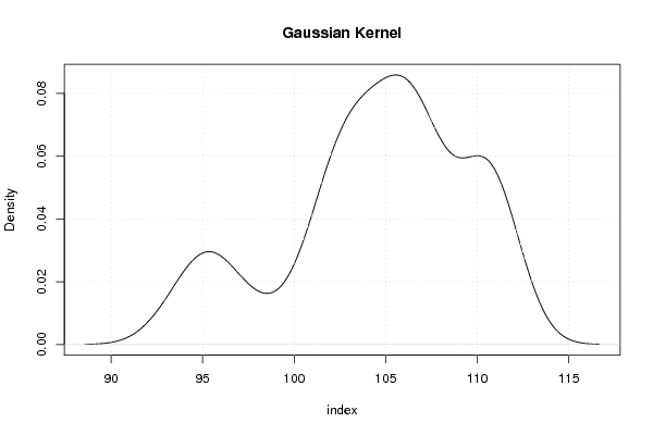
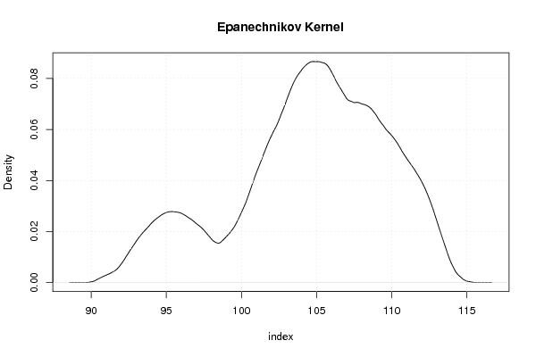
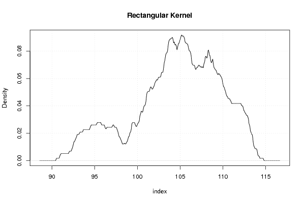
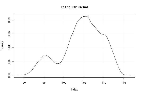
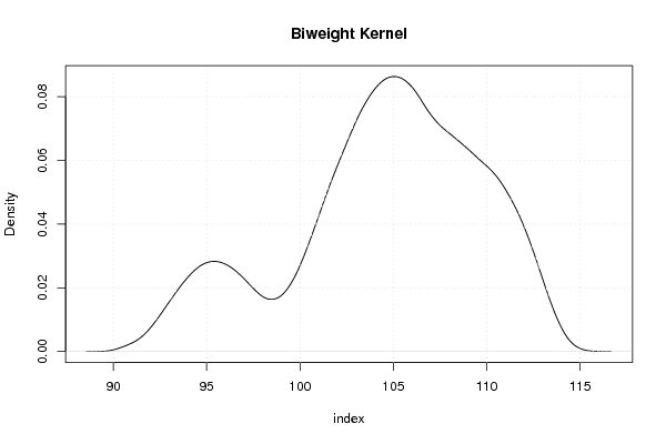
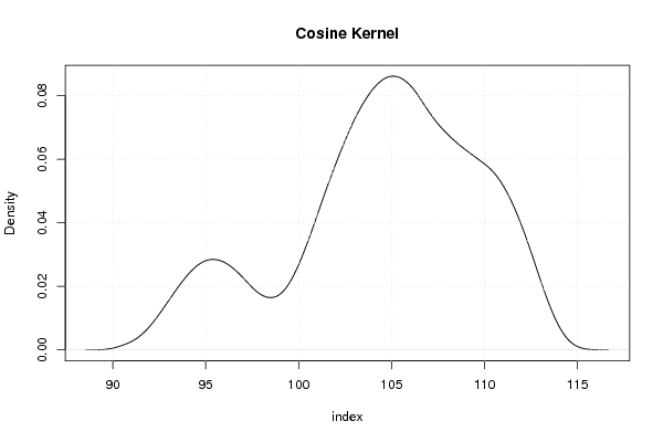
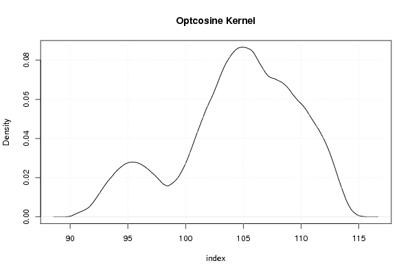
| Title produced by software | Kernel Density Estimation | ||||||||||||||||||||||||||||||||
| Date of computation | Tue, 22 Feb 2011 18:17:39 +0000 | ||||||||||||||||||||||||||||||||
| Cite this page as follows | Statistical Computations at FreeStatistics.org, Office for Research Development and Education, URL https://freestatistics.org/blog/index.php?v=date/2011/Feb/22/t1298398517u2xeiontx9ufqm3.htm/, Retrieved Sun, 19 May 2024 19:08:28 +0000 | ||||||||||||||||||||||||||||||||
| Statistical Computations at FreeStatistics.org, Office for Research Development and Education, URL https://freestatistics.org/blog/index.php?pk=118917, Retrieved Sun, 19 May 2024 19:08:28 +0000 | |||||||||||||||||||||||||||||||||
| QR Codes: | |||||||||||||||||||||||||||||||||
|
| |||||||||||||||||||||||||||||||||
| Original text written by user: | |||||||||||||||||||||||||||||||||
| IsPrivate? | No (this computation is public) | ||||||||||||||||||||||||||||||||
| User-defined keywords | KDGP1W22 | ||||||||||||||||||||||||||||||||
| Estimated Impact | 143 | ||||||||||||||||||||||||||||||||
Tree of Dependent Computations | |||||||||||||||||||||||||||||||||
| Family? (F = Feedback message, R = changed R code, M = changed R Module, P = changed Parameters, D = changed Data) | |||||||||||||||||||||||||||||||||
| - [Histogram] [Marina Cabraja: f...] [2011-02-11 11:36:40] [37062003e6da247d5c55c7deff68feac] - RMPD [Kernel Density Estimation] [marina cabraja: o...] [2011-02-22 18:17:39] [cf9fb0209173b95c2c219e792a280e54] [Current] | |||||||||||||||||||||||||||||||||
| Feedback Forum | |||||||||||||||||||||||||||||||||
Post a new message | |||||||||||||||||||||||||||||||||
Dataset | |||||||||||||||||||||||||||||||||
| Dataseries X: | |||||||||||||||||||||||||||||||||
106,42 106,22 106,32 105,81 105,92 107,54 107,34 107,24 107,74 105,71 105,41 106,22 106,32 106,12 106,22 105,92 105,71 105,71 105,92 105,71 105,41 104,49 101,35 99,72 99,01 97,89 95,86 94,95 95,35 95,15 95,46 95,56 95,05 94,64 93,63 93,12 93,53 97,18 96,27 95,15 97,08 101,95 103,07 103,68 102,87 102,56 103,38 103,27 102,89 102,69 101,54 102,9 101,53 101,96 101,99 101,11 101,75 101,71 104,11 103,57 103,32 103,64 103,68 103,79 103,01 101,54 101,9 103,68 104,62 104,11 105,04 104,83 105,05 104,68 107,32 109,9 109,77 110,69 110,54 110,89 110,95 109,73 110,85 110,39 110,58 110,4 111,07 110,86 111,38 111,44 110,36 110,06 108,34 107,94 107,39 107,1 107,61 107,74 106,9 106,71 106,6 108,21 110,54 110,91 109,51 110,27 111,39 112,13 111,64 | |||||||||||||||||||||||||||||||||
Tables (Output of Computation) | |||||||||||||||||||||||||||||||||
| |||||||||||||||||||||||||||||||||
Figures (Output of Computation) | |||||||||||||||||||||||||||||||||
Input Parameters & R Code | |||||||||||||||||||||||||||||||||
| Parameters (Session): | |||||||||||||||||||||||||||||||||
| par1 = 0 ; | |||||||||||||||||||||||||||||||||
| Parameters (R input): | |||||||||||||||||||||||||||||||||
| par1 = 0 ; | |||||||||||||||||||||||||||||||||
| R code (references can be found in the software module): | |||||||||||||||||||||||||||||||||
if (par1 == '0') bw <- 'nrd0' | |||||||||||||||||||||||||||||||||